Category: today i learned (til)

health, fitness, medicine, environment, ecology, how to learn tricky topics in science and math, new discoveries, news, current events

  • Getting Back to Our Roots:  Using interconnected plant roots as short term data transmitters

    Getting Back to Our Roots: Using interconnected plant roots as short term data transmitters

    I am an Avatar the Last Airbender fanatic. I remember sitting on the couch awestruck watching the final battle between Ozai and Aang. Avatar the Last Airbender never left my heart and I was absolutely delighted to see Netflix’s revival of the show this year. When the Legend of Korra, Avatar’s sequel, was added to the streaming platform, I was overjoyed. During my binging of the fourth season, something perplexing caught my attention. (Do not worry, this contains no spoilers). In one episode, Korra uses the spirit vines to find and communicate with lost children. My fascination exploded and my engineering brain won the “thought-struggle” contest. The premier question: “could plants be used to communicate and send information”? Imaginative thoughts began: tree roots becoming telegraph lines and conducting Morse Code communications. The possibilities of tree root communication would be useful and wonderful, but the biggest obstacle question became apparent: would it work?

    The short answer is, “possibly”, and the reason being is that there are very few studies on the ability of plants to communicate with electricity. Electricity is the basic building block of data transmission. Channeling electricity holds the key to transferring data from one place to another. Current world-wide working channels include optic fiber, copper wires, and Wi-Fi; these channels work by transmitting data by producing electromagnetic signals. The signals carry the information from the output port to the receiving input port. Since plants have an anatomical ability to transmit electricity from their roots to their leaves and vice versa, plants have the potential to be the next transmitting service platform. 

    How plants can transmit data goes back to their roots, literally! Plants are living structures. They are built in three compartments: the root system, the stem, and the leaves. Each part of the plant has separate functions. The roots are used as an anchor in the ground and to soak up molecular nutrients in the soil. The leaves are used to convert sunlight and carbon dioxide into sugars via photosynthesis, and the stem is used as a highway to transport the chemicals and nutrients to the various parts of the plant. While this is basic science, there is a vast oversight on this knowledge. All of what has been said is chemistry. It seems that plants do not use electrical signals in the same way that animals use them. 

    But what does electricity have to do with plants? Similarly to computer data transmissions,  information is sent in electrical signals within plants. Actually, all living beings do this unknowingly, even humans. Every breath taken, hand signal, or step taken requires electrical pulses from the brain to make the movement or action occur. While plants certainly do not walk or make hand gestures, it does seem that they do use electrical signals to send instructions. Some plants like the Mimosa Pudica or the Venus Flytrap  use electrical signals to close their leaves. But, how do normal plants like flowers, trees, and vegetables use electricity?  

    Normal plants do use electricity and electrical potentials to work. In times of droughts, stress, or infections, plants send signals to regulate and try to fix the problem they are experiencing. These messages may originate from any location in the plant; sometimes they originate from an entirely different plant that is connected by their root system. In a study by Annemart Koornneef and Corné M.J. Pieterse (2008), it was found that plants when under attack can cross talk – or talk to plants beside them using the root system as an electrochemical message board. If this interconnected root system can provide a linkage mechanism between plants for them to communicate, then it could be plausible to manipulate the roots to send messages. But this raises the question of can humans manipulate the electrical messaging system? 

    Possibly! One study proved that human applied current on the plant genus arabidopsis, the plant species that are related to mustard and cabbage plants, can conduct current at 3.5 inches per minute. This study confirms that sending man made electrical currents can happen and work, albeit slowly. Yet, the problem lies on the path of travel: the root system. The root systems of trees are interconnected when living in forests or highly populated plant communities. This is because of mycorrhizal fungal connections. The tree roots are not actually intertwined, but are connected by the interconnecting fungi roots that are attached to each individual tree’s roots. An example would be a vast canyon, where the opposing sides are two separate trees and their roots. The mycorrhizal fungi roots act as a bridge connecting the two trees. This bridge acts as a chemical, electrical, and nutrient highway that one tree can use to provide for the other. 

    These mycorrhizal fungi are in nearly every environment in the world. They act as a super highway between hundreds of trees at one time. In a lab setting it was found that mycorrhizal fungi can act as an electrical conductor. The use of these fungi as an electrical forest super-conductor seems to be the perfect setting of a possible natural underground communication and data transfer center. With the entire forest connected by fungi and trees, the plausibility seems to come more into focus. Even in America there are some forests that are so vast that this could be used as a super highway. 

    Take Malheur National Forest in Oregon, where it proudly hosts the world’s oldest and largest organism on Earth: The Honey Mushroom. Estimated to be 8,700 years old, the mushroom covers 940 acres of underground forest floor. The Malheur forest is covered in trees, bushes and ferns, and other plant species, but is all connected by the honey mushroom mycorrhizal network.

    Or consider the Panda in Fishlake National Forest in Utah. The forest is composed of an enormous grove of interconnected Aspen trees, effectively creating one organism. In the forest lies 47,000 nearly genetically identical aspens trees sharing one root system. Spanning 107 acres, Pando – the name of the single Aspen organism – is the largest tree system in the world that spans the same root system. 

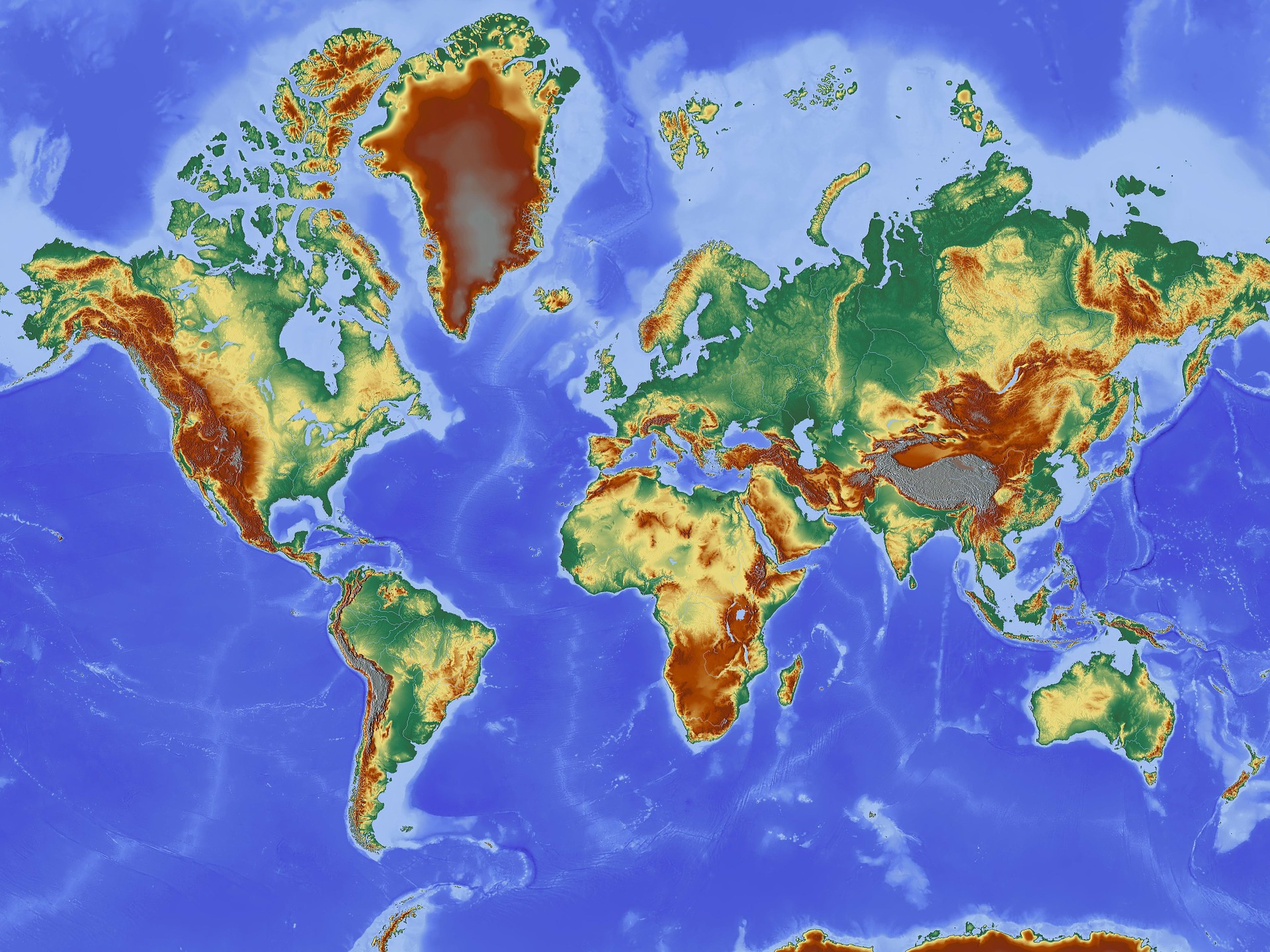
    Beyond North America, think of all the forests in the world: The Amazon in South America, the Congo Basin Forest in Africa, the Sumatra rainforests in Asia, and the hundreds more in Europe and North America. The benefits of implementing and advancing the science of this is world expanding. Some possible benefits for data communication through forest roots include the reduced strain of wireless internet; ecological benefits for increased opposition to deforestation and worldwide planting efforts to rebuild forests. Another benefit is the possible use of discrete non-verbal and non-interceptable communication transfers. Tree root communication has the potential to be used for private and military uses for short range data transmissions. 
    Yet, no task is without its problems. Possible problems that could arise from using this system include lost transmissions from utilizing the wrong root/mycorrhizal pathway; plants and their root systems die and decay, so the cost of upkeep would be massive. Other problems that are the most immediate are that the technology required for this is possibly millions of dollars of research and years away. On both sides of sending the message and receiving the message from a root system is tricky. Beyond picking the pathway, the coding of the message also possesses quite a problem. All these problems are significant roadblocks, but can ultimately be overcome with science, engineering and time. 

    I personally believe that tree root data transmission would and could be of significant use with endless possible benefits. Hiking in the woods with no cell reception? Just tap into a tree and place out a distress call! In quarantine and want to talk to someone in your wooded neighborhood? Send out a tree root instant message! My first thoughts were using tree roots with Morse code or even how farmers in the great depression used their barbed wire fences as communication devices. The root system communication and data transfer would expand and grow over time as more and more forests mature and grow. A future where you could tap into a pine tree and dial up your neighbor down the street may seem foreign, but in the future, calling, texting, sending memes and gifs, or encoded data plans may be a possibility. 

    It all goes back to finding our roots. 

    References

    • Gebelhoff, Robert. “Plants Send out Stress Signals Just like Animals, Scientists Find.” The Washington Post, WP Company, 28 Apr. 2019, www.washingtonpost.com/news/speaking-of-science/wp/2015/07/30/plants-send-out-stress-signals-just-like-animals-scientists-find/.
    • Jabr, Ferris. “Plants Cannot ‘Think and Remember,” but There’s Nothing Stupid about Them: They’re Shockingly Sophisticated.” Scientific American Blog Network, Scientific American, 16 July 2010, blogs.scientificamerican.com/observations/plants-cannot-think-and-remember-but-theres-nothing-stupid-about-them-theyre-shockingly-sophisticated/.
    • Nield, David. “Plants Can Secretly Send Underground Electrical Signals. Here’s How They Do It.” ScienceAlert, Communicative & Integrative Biology, 14 July 2020, www.sciencealert.com/here-s-how-plants-can-secretly-send-each-other-underground-electrical-signals.
    • Thomas, Brian. “Shocking Evidence of Electrical Signals in Plants.” The Institute for Creation Research, The Institute for Creation Research, 11 Sept. 2013, www.icr.org/article/shocking-evidence-electrical-signals.
    • Yoon, Carol Kaesuk. “Plants Found to Send Nerve-Like Messages.” The New York Times, The New York Times, 17 Nov. 1992, www.nytimes.com/1992/11/17/science/plants-found-to-send-nerve-like-messages.html.

  • Three Dog Star Night (Part 1)

    Three Dog Star Night (Part 1)

    I am just old enough to remember a time when most textbooks only spoke of exoplanets (i.e. those outside our solar system) in the hypothetical sense, their existence taken as an assumption rather than demonstrable fact, while the question of whether our 8-planet solar system was typical or an anomaly remained a hotly-debated topic. Despite over a century of attempts and subsequent erroneous claims, it wasn’t until 1992 that the first confirmed exoplanet was discovered, two of them as a matter of fact, orbiting the pulsar PSR B1257+12. As surprising as this was to the scientific community, the high likelihood that the planetary pair had formed as the result of a merger between two white dwarfs rather than a collapsing gas cloud meant the world would have to wait another 3 years for the confirmation of a “true” planet orbiting a main-sequence star like the Sun. The discovery ushered in a new era for astronomy and as of November 1st, 2020 there have been a whopping 4,370 exoplanets confirmed in 3,230 star systems. This menagerie of other worlds, ranging from “hot Jupiters” and lava worlds to gas and ice giants and seemingly everything in between stands in stark contrast to the apparently silent heavens, leaving a profound question unanswered:

    “Where is everybody?”

    Despite what many a crackpot relative or internet crank will tell you, humanity is, to the best of our knowledge, completely and utterly alone in a universe so vast it defies comprehension, a contradiction commonly referred to today as The Fermi Paradox. The concept of aliens and the foundations of the Fermi Paradox have been around for a surprisingly long time, entering the Western conscience with the speculation of Epicurean philosophers like Democritus of ancient Greece, who today is famous for the first conception of atoms. From the viewpoint that the world was merely a chance jostling of these atoms, they argued it was not only reasonable, but exceedingly likely that there exist other inhabited worlds similar to our own. To paraphrase the argument: “who ever heard of a single ear of wheat growing alone in a vast, fertile field?”

    Should you happen to see this mentioned on the next episode of Ancient Aliens, it’s worth noting that Democritus’s ideas about “aliens” (and atoms) are not quite as modern as they sound, instead more akin to our modern idea of beings from “parallel universes”, not habitable planets orbiting other stars since the ancient Greeks had no idea what stars and planets actually are, much less orbits. To them, these other worlds existed but were forever inaccessible to us. What’s important is that the core idea, that it’s improbable that life should arise on Earth and only on Earth begins here. Its dismissal by the Aristotelians, who preferred what can be known to what might be and whose influence on Western culture remains to this day, caused such discussion to take a back seat during the early Middle Ages, but the idea remained nonetheless, never being fully dismissed as “impossible” by theologians who were wary of placing what they saw as limits on the omnipotence of the Christian God. Contrary to the popular misconception that discussion of such matters would get one labeled a heretic and burned at the stake, the idea of aliens inhabiting other worlds within our universe that were, at least in theory, accessible to us in some way first arose in the Western world during the late Middle Ages. In his influential work De Docta Ignorantia (1440), Nicholas of Cusa argues that:

    Life, as it exists on Earth in the form of men, animals and plants, is to be found, let us suppose in a high form in the solar and stellar regions. Rather than think that so many stars and parts of the heavens are uninhabited and that this earth of ours alone is peopled – and that with beings perhaps of an inferior type – we will suppose that in every region there are inhabitants, differing in nature by rank and all owing their origin to God, who is the center and circumference of all stellar regions (II, p. 12).

    His work sparked intense discussion among Christian theologians over whether or not such aliens had been “redeemed” and even whether “original sin” would apply to them. After all it was probably a safe assumption that they were not descended from the mythical Adam and Eve.

    The idea stuck around and was eventually taken up by the scientists of the modern era, including the likes of none other than Harlow Shapley who stated in an interview for The Sydney Morning Herald (1959) that:

    The universe has 10 million, million, million suns similar to our own. One in a million has planets around it. Only one in a million million has the right combination of chemicals, temperature, water, days and nights to support planetary life as we know it. This calculation arrives at the estimated figure of 100 million worlds where life has been forged by evolution (p. 5)

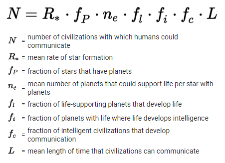
    Five months later, Frank Drake performed the first systematic search for extraterrestrial intelligence by monitoring two nearby sun-like stars, 6 hours per day for four months, searching for radio signals around the emission frequency of neutral hydrogen, the most common element in the universe. The reason for this frequency choice is simple: if somebody out there wants their message to be heard, they’ll put it where everyone is already looking. A year later, while preparing to host a meeting for SETI to discuss the future potential of such search efforts, he penned the equation which would bear his name.

    Though initially conceived as little more than a mathematical conversation piece, The Drake Equation (as it came to be known) at last allowed astronomers to estimate the number of intelligent civilizations within our galaxy, for the first time couching the discussion in numbers rather than idle speculation. The only problem? Nobody had any real idea what any of these numbers actually were. The various numbers proposed at the meeting by Drake and his colleagues as an “educated guess” give a final value somewhere between a minimum of 20 and a maximum of 50,000,000. Such an enormous range perfectly illustrates their aforementioned uncertainty. In the six decades since, the data from countless observations, surveys, and space missions from NASA, ESA, and observatories around the world have finally shed some light on a few of these parameters which, in theory, allow us to narrow down the estimates a bit.

    Mean Rate of Star Formation, R*

    Our first parameter in the Drake Equation is R*, the average rate of star formation. For our purposes here, we are only looking for life within our own galaxy so we will use the rate of star formation in the Milky Way. Calculations from the available data suggest that somewhere between 0.68 and 1.45 solar masses of galactic material goes into making new stars every year. To find the star formation rate, we need to also account for the average mass of new stars using the available empirical data which indicates a value of around two stars per solar mass worth of material. Multiplying these two numbers together gives us a value between 1.5 and 3 new stars per year formed in our galaxy, a value slightly higher than the original 1961 estimate of 1 per year.

    R* = 1.5 – 3

    The Fraction of Stars that have Planets, fp

    As mentioned previously, the exoplanet surveys thus far found 3,230 star systems that contain planets. However this figure only tells us the number of stars that have been found to possess planets, not the fraction of them that do. The total number of stars surveyed is much larger at over half a million. Dividing the two numbers gives a value for fp of less than 1%. At first glance, this looks pretty dismal, but there are some important caveats that we need to account for. The majority of exoplanet discoveries were made using the transit method, which makes continuous observations of a star’s light to look for periodic dimming caused by a planet passing in front of it directly along our line of sight. Our chances of observing such dimming is directly related to the star’s radius (bigger is better) and inversely related to the planet’s orbital distance from its host star (closer is better). Should our line of sight to a given system happen to be anything other than virtually edge-on, the transit method will not detect any planets there, even if there actually are. For those that we are fortunate enough to be observing nearly edge-on, if a planet’s orbit is too wide then it will not pass in front of the star from our perspective, thus there will be no dimming and the planet will go undetected. Finally, if a planet is too small, then the star’s dimming could be too small for our instruments to detect and the planet will go undetected.

    It perhaps seems that we’re out of luck on getting any reasonable estimates, but statistical analysis of the transit data combined with that of surveys using other methods of planet detection such as doppler spectroscopy and gravitational microlensing point towards a conclusion that even the optimists of the 1960’s would consider absolutely astonishing; fp may very well approach 1, far larger than the maximum estimated value of 0.5 made 60 years ago! In other words, it’s possible that nearly every single star in our galaxy has one or more planets!

    fp ≈ 1

    Thus far things are looking better than ever for the potential development of intelligent, detectable civilizations (IDCs) in our galaxy, only deepening the paradox. However from here on our estimates for successive factors in the Drake Equation become increasingly speculative.

    The Fraction of Potential Life-Supporting Planets that Develop Life, fl

    This number is even more difficult to estimate than the previous factor. Our current sample size for life-supporting planets that go on to develop life is 1, with a possibility of 5 more if Mars, Venus, Titan, Europa, and/or Enceladus are eventually found to have or have had life. Some scientists argue that life arises as a rule virtually as soon as conditions are right, so this value should be ‘one’. Others argue it may actually be a freak occurrence even in all the right conditions, so this number should be tiny. In the case of our planet, life appears to have developed as soon as the conditions were right, but any attempt to extrapolate this to other planets contains heavy anthropic bias as our model planet (Earth) was not chosen randomly but rather by the organisms already inhabiting it. There currently is no evidence that abiogenesis occurred more than once on Earth, yet if it were a common phenomenon we might reasonably expect it to have occurred several times. It certainly could have, but all known terrestrial life shares a common origin, meaning if it ever did then those lineages are most likely long gone. If abiogenesis does indeed turn out to be an incredibly rare event, there is still a potential loophole. Remember, we only care about the number of habitable planets that go on to actually develop life, not how that life got there in the first place. It is entirely conceivable that planets, including our own, could have been seeded with microbial life that hitched a ride on a rogue piece of post-collision debris ejected from another already inhabited planet, a hypothesis known as panspermia. A technologically advanced civilization could also choose to do this intentionally in order to spread its genetic family throughout the galaxy. It may sound far-fetched, but humanity already has the capability to do this. Scientists and engineers go to painstaking lengths to sterilize spacecraft in order to avoid unintentionally ‘infecting’ other planets or moons with potentially invasive extremophile Earthlings. The various proposed panspermia hypotheses are a topic that honestly deserve an article all their own, so for now we will wrap things up optimistically and use the original estimate made by Drake and his colleagues back in 1961.

    fl ≈ 1

    You may have noticed we skipped over a factor, the average number of habitable planets per star with planets. Like panspermia, this factor warrants its own discussion and is the subject of part two in this series. Stay tuned!

  • Three Dog Star Night (Part 2)

    Three Dog Star Night (Part 2)

    Welcome back to our discussion on the Drake Equation and the Fermi Paradox! If you haven’t read part 1 already, it goes without saying that you should start there! This time around, we will be discussing what we know about habitable planets… or at least what we think we know. Strap in, friends. This is going to be a long one.

    Before we proceed any further we need to introduce the concept of ‘filters’, i.e. factors that may inhibit the development of life and, ultimately, intelligent, detectable civilizations (IDCs) on a given planet. It is crucial to keep in mind that all proposed filters are not absolutes, rather they are speculative reasons why IDCs may be rare, thus resolving the Fermi Paradox. For convenience we can designate “Lesser” filters as those which eliminate 0% to 50% of all planets, “Minor” filters which eliminate 50% to 90%, “Major” filters which eliminate between 90% and 99.9999%, and finally “Great” filters which eliminate 99.9999% to 100% of planets. With this caveat in mind, we move on to our next parameter in the Drake Equation.

    The Average Number of Habitable Planets per Star with Planets, ne

    In order to determine what types of planets can support life, we first need to know what conditions are actually right for life, a difficult task given our current sample size of one. Of the eight planets in our solar system, only Earth is known to host any life at all. Though the emerging field of astrobiology is beginning to shed new light on the issues of whether or not life could have existed on Mars and Venus in the past or concurrently in the subsurface oceans of moons like Enceladus and Europa, the question remains open. Note that we are only looking for planets with the potential to support any life for this number, be it microbial or otherwise. We certainly do not expect microbes to start sending messages out into space, but the distinction between life and intelligent life is one that will be accounted for by subsequent numbers in our equation. This will allow us to save many of our potential filters for later and simply focus on habitability in all its possible forms. Sadly, those that remain are the ones we are most certain about.

    We can begin to approach the problem by flipping it around, instead asking the reverse, “What conditions preclude life from developing?” If we focus exclusively on planets, our sample size has septupled since there are seven planets in our solar system that are known to not support life. Investigating the factors that prevented life from existing for a significant amount of time provides us with some starting filters which allow us to eliminate entire swaths of planets from the veritable zoo of those discovered.

    Filter 1 – Location, location, location!

    The clichéd real-estate adage provides us with our first filter. Since we are focusing solely on the Milky Way, we don’t need to worry about galaxy type. Our own existence is proof that our galaxy is among those that are right for hosting life, so we need not concern ourselves with filters like active galactic nuclei, galaxy mergers, etc. However many astronomers propose that a star system’s location within a galaxy is an important factor. There may very well be a so-called “habitable zone” on the galactic scale in addition to that found around the individual stars themselves. Close to the crowded galactic center a system is likely to be subjected to nearby supernovae, migrating black holes, asteroid/comet impacts, passing pulsars, and other devastating natural phenomena with the potential to sterilize entire planets. On the other hand, systems at the galaxy’s edge are unlikely to have enough nearby gas and dust to sufficiently drive the formation of stars and planets. The average stellar metallicity (how much of a star is composed of elements heavier than helium) declines as distance from the center increases, so stars near the galaxy’s edge are expected to have fewer rocky, potentially life-sustaining planets. As it turns out, this may not ultimately be the case as some data suggests rocky planets could be more common around lower-metallicity stars, but for now this will be our working assumption.

    This limits the expected life-sustaining region of our galaxy to stars whose orbits lie from at least 1 to at most 10 kiloparsecs from the center. For reference the Milky Way has a radius of only about 15 kiloparsecs, and with a little data and some rough assumptions, one can calculate that only around 10% of all stars in our galaxy lie in this region. This number is still staggeringly large and includes, to first order, around 20-40 billion stars or so. Of those we can reasonably exclude the 10% of stars in our galaxy that are not on the main sequence. Given that the average number of planets per star may be as high as 10 on the extreme optimistic end, this leaves a maximum of about 360 billion planets to work with.

    In addition to the galaxy, the stars themselves each have their own habitable zones, defined as the range of orbital distances within which liquid water could conceivably exist on the surface in large quantities. There are only three planets in our solar system that exist more or less within the sun’s habitable zone: Venus, Earth, and Mars. Of these three, Venus and Mars are each close to the edge of what can be considered the habitable zone, and given the concept’s speculative nature these boundaries could grow or shrink with new information. The most we can do right now is place an upper limit on this value of 6, based on research by Dr. Christa Van Laerhoven and her colleagues, though the actual number is almost certain to be lower. For simplicity, we can estimate the average number of planets in a star’s habitable zone to be 3. The size and location of the habitable zone is determined by the type of star. Large stars (O, B, and A types) account for only about 7% of all stars and tend to burn out too soon for complex life to really gain a foothold. It’s uncertain whether planets around smaller, red dwarf stars might host life. The data indicates the planets orbiting in their habitable zones may be tidally locked to the star just as the moon is to the Earth, with one side facing the star at all times. While this doesn’t preclude life from forming, it certainly makes things more difficult. Red dwarf stars may account for as much as 75% of the stars in our galaxy, so whether they should be included in the search for life is a crucial question that will hopefully be answered as more data becomes available. Nonetheless we have our next filter: of the main sequence stars, at most 93% of them are expected to be habitable.

    There are without a doubt more particulars of planetary arrangement that come into play here, such as having a stable, mostly circular (low eccentricity) orbit, the role gas giants like Jupiter may play as cosmic vacuum cleaners, and more, but the only thing we know for sure regarding the rest of the Location Filter is that we just don’t know.

    Filter 2 – Earth-Sized:

    Planets that are too large tend to be gas or ice giants, with no solid surface and crushingly thick and turbulent atmospheres. Life could form here, but if it does, it’s likely the exception rather than the rule. At the same time, the cores of planets that are too small tend to cool too quickly and lose their magnetic fields and subsequently their atmosphere to stellar winds. Mars is a perfect example of this. Looking at the best current estimates, we can see that only around 1,237 of the 4,370 exoplanets discovered so far are “Earth-sized”, i.e. range from 0.8 to 2 Earth radii. We can be generous here and allow for the fact that exoplanet survey methods are biased towards larger planets by estimating that perhaps 40% of planets are Earth-sized.

    Filter 3 – Atmospheres, Plate Tectonics, and Moons:

    Being Earth-sized helps when holding onto an atmosphere, but this does us no good if it isn’t the right atmosphere, and we need look no further than our own solar system for the perfect illustration of this. Venus is 93% the mass of the Earth, yet its atmosphere is crushing at a choking 100 times the density of Earth’s. Unlike our own atmosphere which is about 70% Nitrogen, Venus’s atmosphere is more than 96% CO2, 30 times the CO2 concentration of our own atmosphere. This runaway greenhouse effect famously makes Venus the hottest planet in the solar system, with surface temperatures hot enough to melt lead. Unfortunately we have no real data for this yet as we lack the ability to reliably observe exoplanet atmospheres, though that is expected to change with the launch of the James Webb Space Telescope set to launch in October of 2021. For now, we will be generous and use our own solar system as the model by assuming that 50% Earth-sized planets do not have the right atmosphere for life.

    Two other factors that make Earth, well, Earth-like are plate tectonics and our Moon. Plate tectonics play a crucial role in cycling numerous elements, including carbon and phosphorus, in and out of the environment. It’s thought that Earth’s water and the theoretical collision with a Mars-sized planet which formed the moon are two of the main factors that got plate tectonics going. Venus, which lacks both, shows no signs of tectonic activity, past or present, even though its core is known to still be molten and active. The Moon is somewhat of an anomaly in its own right. Of all the planetary moons in the solar system, it is by far the largest relative to the size of its host planet. Its existence helps to stabilize Earth’s axial tilt and over billions of years, through a quirk of angular momentum conservation, gradually slowed our planet’s initially brisk rotation to the 24 hour day/night cycle we experience today. It also generates tides and thus tidal pools, which some theories for abiogenesis claim provided the conditions for the origin of life on the early Earth. Again, we will be generous here and presume that 1 in 2 Earth-sized planets in the habitable zone of their star are actually Earth-like.

    Filter 4 – Phosphorus Scarcity:

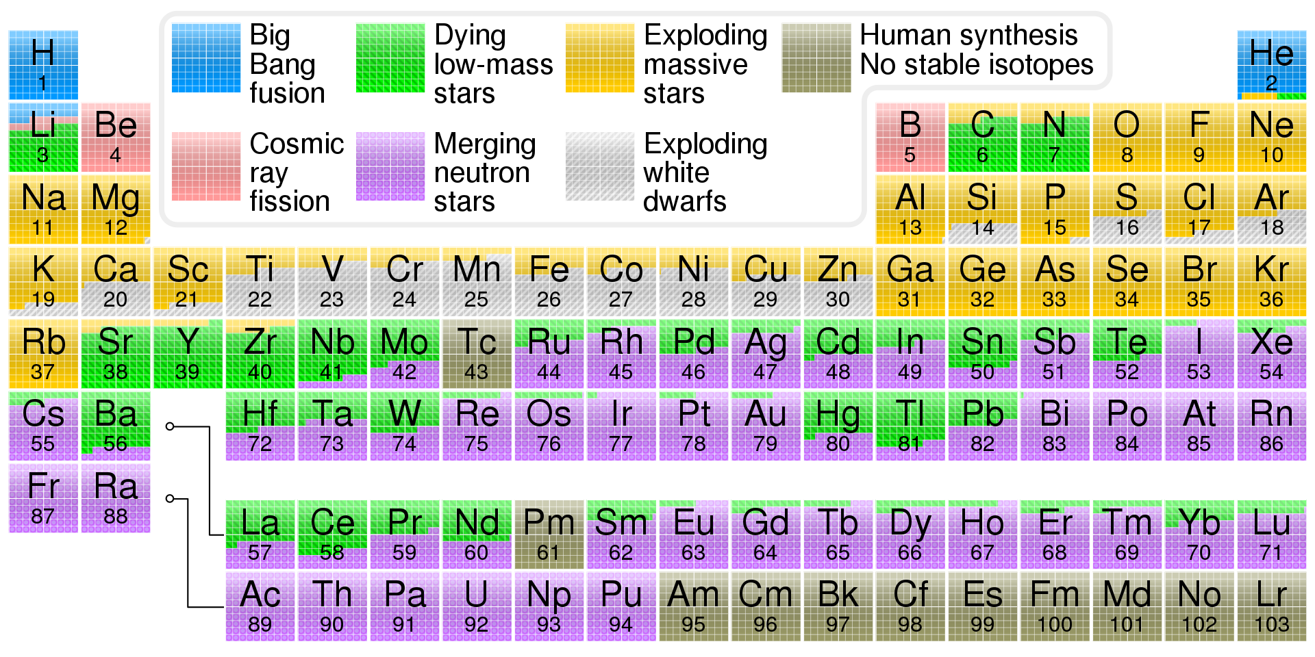
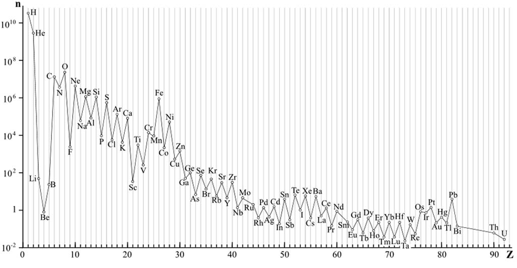
    A recent study of two supernovae remnants, the Crab Nebula and Cassiopeia A, by Dr. Jane Greaves of Cardiff University and her team suggests that phosphorus may be produced in vastly different quantities during supernova nucleosynthesis. It’s somewhat common knowledge, even among the general public, that the Big Bang produced only Hydrogen, Helium, and a possibly a small amount of Lithium, and that all elements higher on the periodic table were produced in the cores of stars as byproducts of nuclear fusion, a process known as hydrostatic burning, but this is only half of the story. Stellar nucleosynthesis can only account for the production of a specific set of elements, most of which have an even number of protons due to their fusion being reliant on Helium and none of which are heavier than Zinc (element 30). All elements with more than 30 protons can only be naturally produced by what happens after stellar nucleosynthesis ends, in the explosive deaths of stars and the violent collisions of their remnants. As the star collapses infalling matter piles up and is “bounced” back out, producing large numbers of neutrons and sending shockwaves through the star’s layers which quickly fuse lighter elements into heavier ones through the process of rapid neutron capture, known as the r-process. In fact the majority of the elements trace their origins to events beyond the cores of main sequence stars as can be seen in the chart below. All of this results in massive discrepancies in universal abundances between elements, shown in the second image. Taking particular note of what the data shows regarding the six elements considered most critical for life: Hydrogen, Carbon, Nitrogen, Oxygen, Phosphorus, and Sulfur. Phosphorus in particular is required for the metabolic processes of all known cells (via ATP) and forms the backbone of both DNA and RNA, yet it is by far the least common of the six.

    (By Cmglee – Own work, CC BY-SA 3.0, https://commons.wikimedia.org/w/index.php?curid=31761437, based on data by Jennifer Johnson at Ohio State University)

    The most likely production process involves a silicon-30 isotope capturing a neutron during the supernova, briefly becoming unstable silicon-31 before one of its neutrons emits an electron and an antineutrino to decay into a proton, transmuting the atom into phosphorus-31, the element’s only stable isotope. The problem is that silicon-30 is not the most abundant Si isotope, accounting for only about 3.1% of all naturally-occurring Silicon, and its cross-section for neutron capture is quite small, meaning a neutron has to hit it just right to get absorbed. Supernovae are not evenly distributed around the galaxy, and thus we already expect that phosphorus isn’t either. Should it be the case that Phosphorus is not a ubiquitous byproduct of supernova nucleosynthesis, the element will only be rarer and more unevenly distributed than previously thought. There could very well be entire swaths of the galaxy with virtually none at all.

    While it might be possible for life to develop that does not rely on phosphorus, the chances of that actually happening are probably slim, and such life would be the exception rather than the rule. We ourselves are composed of approximately 1% phosphorus, the planet’s crust is about 0.1% phosphorus, and the entire solar system is roughly 0.0007% phosphorus by mass. On the scale of the entire universe, phosphorus only accounts for about three of every ten million atoms, or 0.00003%, and would have been even lower than that when our solar system began to form 5 billion years ago. Naturally, older star systems are expected to have less phosphorus on average as fewer phosphorus-producing supernovae would have occurred prior to their formation. Even our apparent relative abundance of phosphorus is so low that it presents a problem for scientists seeking to tease out the origins of life. Phosphorus also tends to bind into molecules that are heavier and thus would have sunk towards the core during the planet’s formation, though the collision which we think formed our Moon may have played a role here in dredging some up from the Earth’s interior. Its common compounds also tend to be insoluble in water which is problematic since life processes are pretty much predicated entirely on water solubility. Unlike the Earth’s carbon cycle which is relatively quick on geological timescales and involves the atmosphere as well as the planet’s interior, the phosphorus cycle is one of the slowest and independent of the atmosphere, so biologically-available Phosphorus is only refreshed by tectonic activity. That life should rely so ubiquitously on phosphorus despite its apparent scarcity tells us either that phosphorus-based life is easier to form than non-phosphorus-based life or that life based on phosphorus has an evolutionary advantage over life that is not. Possibly even both. Water is quite common in the universe, and so it may be that Phosphorus is what makes Earth truly unique among the planetary zoo.

    Until there is conclusive evidence one way or another, we can take this potential filter with a grain of salt and estimate that only 50% of planets have a sufficient amount of Phosphorus present on the surface. We can now combine all our filters into one to calculate a final value for ne and find that several Lesser and Minor Filters have combined to form one Major Filter. With less optimistic estimates, such as excluding red dwarf stars, and a few more assumptions and factors accounted for, this has the potential to reach Great Filter status and serves as the foundation for the Rare Earth Hypothesis.


    ne, Optimistic = 3 x 0.1 x 0.9 x 0.93 x 0.4 x 0.5 x 0.5 x 0.5 = 0.0125

    ne, Rare Earth < 0.000001


    For now, this is where we will leave the second half of our discussion of Drake’s equation. We can take all the factors we’ve discussed so far, multiply them together, and multiply this value by the length of time life has existed on Earth (3.5 billion years) to get a somewhat crude estimate for the number of planets in the galaxy which might contain life in any form.

    NOptimistic = 131,250,000

    NRare Earth < 10500

    When compared against the hundred billion or so planets that are estimated to reside within the Milky Way, even our deliberately generous estimate indicates that only around 0.13% of planets harbor any life at all. If we apply the Rare Earth filter for ne, then only about 0.00001% of planets in the Milky Way are safe havens for life. These numbers will only diminish as we start accounting specifically for intelligent life in subsequent factors of the Drake Equation. After all, the Fermi Paradox is specifically about why we haven’t heard from any other intelligent life, not merely the chances that extraterrestrial life in general exists.

    Next time we’ll be discussing that second half of the Drake Equation and the implications further proposed filters have for our chances of detecting intelligent life within the Milky Way. Unfortunately, the last three factors rely heavily on speculation in the absence of virtually any reliable data, and we will delve deep into some of that speculation in part 3. In part 4 we’ll discuss the final factor of the equation and run some example calculations before finally delving into what the Drake Equation actually is. In the meantime, if you’d like to try your hand at estimating the number of inhabited planets or intelligent civilizations in the universe, you can use this handy link for calculating the Drake Equation.

  • Can diapers improve agricultural management?

    Can diapers improve agricultural management?

         Ever wondered how diapers can hold and absorb so much liquid?  The simple answer is hydrogels.  Disposable diapers have been on the rise in popularity in recent years because of their ease of use.  Unfortunately with the sudden increase in popularity of diapers,  waste management is a big issue all around the world.  Everyone is trying to find new and innovative ways to decrease the generation of waste.  Because of the short life span of disposable diapers, they end up in a waste field which causes very serious environmental impacts. Consequently, people are switching over to reusable diapers.  While this is, in fact, a positive, the much bigger issue is in developing countries where the majority of disposable diapers are being used.  In many of these developing countries, the used diapers are disposed of in either landfills or open dumpsites.  The mismanagement of solid waste can lead to an increase in greenhouse gas emissions and water pollution from the open dumpsites.  These hydrogels after being sanitized might have the possibility to be reused or repurposed for another product.   Current research focuses on the reuse of hydrogels for soil irrigation.  

         A hydrogel is a chemically or physically bonded polymer.  Chemically bonded hydrogels are permanent and chemically cross-linked together.  Physically bonded hydrogels are reversible and are held together by hydrogen bonding from its interactions with water.  The only difference between chemically and physically bonded hydrogel is that physically bonded hydrogels can be separated into individual components.   How much water a hydrogel can hold is the point of equilibrium swelling which is the most important characteristic.  When a hydrogel connects with water, the hydrophobic groups interact with the water molecules. The hydrophobic group tends to repel water, which leads to the swelling of the hydrogel.  As the hydrogel swells, it is absorbing the surrendering water until it reaches its equilibrium swelling point.  Every hydrogel has its own equilibrium swelling point.  Once it reaches this point it will not swell anymore and the additional water will fill in the spaces between the bonds. 

          Traditionally, agricultural methods are based on irrigation methods such as drip and spray and, flood irrigation.  This has some downfalls because not all the water is absorbed by the plants which can lead to runoff water.  In some countries, this poses a bigger threat because of the scarcity of water.  Sandy soils are impacted at a greater extent because they have low water carrying capacity which makes it hard for them to absorb water.  This leads to most of the water being unabsorbed and the plant roots lacking sufficient water and nutrients.  Since hydrogels are very absorptive,  they can be used to absorb some of the excess water so the water does not go to waste. 

         Hydrogels can be used to improve agricultural management.  Many studies are looking into if the hydrogels in diapers can be reused and repurposed after sanitation, but still, maintain the level of equilibrium swelling and have the ability to hold the water for a long period of time. Luckily, they were proven to have a larger equilibrium swelling capacity and a longer swell time.  These two factors can greatly improve water retention in soil and irrigation efficiency.  Because of the basic properties of a hydrogel, they are allowed to slowly release the water back into the soil, this allows improved water efficiency.  This is because the plant’s roots are not drowning in large amounts of water which makes it harder for them to retain all of it.  While the hydrogel is in the soil, it will wrap around the roots and will continue to give the roots the water supply it needs for photosynthesis.  There still is a long way to go on researching this idea, but maybe in the future, we will be able to reuse hydrogels and many other everyday items.  

    Citations 

    Agaba, H., Orikiriza, L., Obua, J., Kabasa, J., Worbes, M., & Hüttermann, A. (2011, November 17). Hydrogel amendment to sandy soil reduces irrigation frequency and improves the biomass of Agrostis stolonifera. Retrieved November 24, 2020, from https://www.scirp.org/journal/PaperInformation.aspx?PaperID=8549

    Al-Jabari, M., Ghyadah, R., & Alokely, R. (2019, March 20). Recovery of hydrogel from baby diaper wastes and its application for enhancing soil irrigation management. Retrieved November 23, 2020, from https://www.sciencedirect.com/science/article/pii/S0301479719303901

    Ferronato, N., Nova Pinedo, M., & Torretta, V. (2020, June 21). Assessment of Used Baby Diapers Composting in Bolivia. Retrieved November 24, 2020, from https://www.mdpi.com/2071-1050/12/12/5055

    Zekry, M., Abdallah, A., Salim, H., & Nassar, I. (2020, March 07). The Potential of super absorbent polymers from diaper wastes to enhance water retention properties of the soil. Retrieved November 24, 2020, from https://www.researchgate.net/publication/341756185_The_Potential_of_super_absorbent_polymers_from_diaper_wastes_to_enhance_water_retention_properties_of_the_soil


  • Insect robots: How do they fly?

    Insect robots: How do they fly?


    “How do airplanes stay afloat?”

    “The same way a bird stays afloat.”

    When we give that answer to a kid, we fondly realize the connection between nature’s creatures and machines, and that the nature influenced creation of many machines from time to time. That is why the Wright brothers spent a great deal of time observing birds in flight and realized that when birds soared into the wind, the air flowed over the curved surface of their wings, and thus generated lift which helps them stay in flight. They noticed the wings of birds minutely, and realized that they change the shape of the wings to turn and maneuver, and thus flaps and stabilizers were born in the airplane wings. In a similar fashion, various insects and birds have influenced designs of many machines for their structural and aerodynamic ability. These creatures not only helped design the structural and aerodynamic systems of large machines, but attracted considerable attention from scientists and engineers for small-scale robots. Today we deep dive into the world of small robots and how they fly!

    Insects were the first organisms on Earth to take to the skies – estimates on the origin of insect flight range from ~320 to ~400 million years ago (Misof et al., 2014). That is a long, long time before vertebrates achieved this feat. Over time, insects mastered their flying ability, and achieved great perfection in speed, agility, and grace in the air. By design, insects such as hover flies and birds such as hummingbird have remarkable abilities to hover in the air, as well as being able to perform aerobatic maneuvers such as sideways or backward flying. The technique that they use is called a flapping wing motion. This remarkable ability is a key in the design of small-scale aircraft for surveillance or reconnaissance. Traditionally, engineers designed a medium to large scale aerodynamic vehicle with traditional mechanical linkage systems (Van Breugel et al., 2008). However, when it comes to an unmanned small-scale aerial vehicle (or even micro-scale that mimics the size of an actual small insect such as a hover fly), one of the key challenges in traditional designs was that the flapping-wing action was not stable because of the power and weight ratio that needs to be achieved to match the hovering and flying abilities of the insects and birds observed in nature.

    Historically, there have been a number of research efforts that focused on the mechanical and structural aspects of a small-scale flying robot design. One such project was the Entomopter project in Georgia Tech (Michelson et al., 1998). The researchers used a chemical muscle to produce linear actuation strain. Two sets of rigid wings (front and back) were placed, and chemical muscle actuated them. Other traditional designs of small-scale flying robots used gears and links for the movements needed for of an airborne vehicle.

    How do the “insect” robots get up in the air?

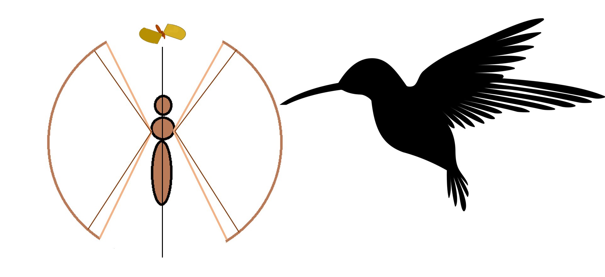
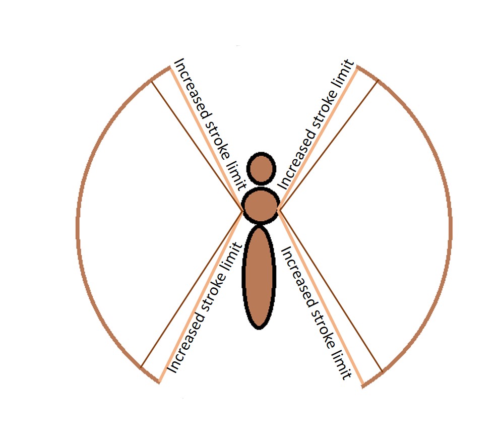
    In order to achieve a flapping action in-flight to gain altitude, sweeping and the pitching motions are needed to be achieved. The current design is set up to exploit resonant properties, as exhibited by flying insects, to reduce the energy expenditure and to provide amplitude amplification for the wing sweeping motion (Bolsman, 2010). Design objective for a small-scale flying machine is to reproduce a reference motion based on the kinematics of insects. Insects and birds perform wing flapping and adjustments of the body orientation in order to control speed, altitude and orientation of the flight. As shown in the figure below, to transfer this analogy to a micro-robot, the sweeping motion of the wings are emulated as a steady-state motion. The details of a control system can be found in advance literature (Bolsman, 2010). However, in simple terms, the design takes into account a constant resonance frequency, and a maximum wind sweeping stroke. As the stroke increases (shown by the extreme lines in the figure), the wings generate lift. The mass of the device (as in an insect) is centered towards the geometric center of the device, resulting in maximum possible stability. This is the stage where the robots get airborne and continue hovering.

    Lift: Flapping wing motion with sweeping stroke

    How do the “insect” robots move in the air?

    The hovering is the first state of condition that the robots achieve, similar to an insect. The figure above shows a simple two wing device. Each wing is designed to have independent controls to change flapping In order to change the direction to left or right, so that each wing is capable of having a different sweeping motion. This inevitably creates a sweeping motion that are not equal in each wing, and results in a rotation in the direction of the difference. An insect performs these exact same maneuvers to create a rotational motion for left-right (rolling) movement.

    As shown in the figure, the center position holds the center of mass for the whole assembly. As such, changing the center position of the sweeping motion will change the direction of flight as well. This is performed by shifting the positions of the effective centers of pressure of the left and right wings. This invariably creates a backward motion (or pitch), and more power from the device’s power source provides a required forward motion while maintaining the achieved altitude.

    How strong are these “insect” robots?

    A simple model of a small-scale flying robot has been described here to depict the fundamentals that are derived from an insect or a small bird for flapping motion design. A fully fledged flying micro robot has more control systems that are able to achieve a full range of motions if needed, with more complicated actuations that are associated with multiple wings and wing rotations. In addition, structural integrity is also a key factor which, surprisingly, is also derived from insects. One of the most fascinating and extraordinary creatures in earth are ants, they can carry objects several times of their body weight. Ant’s neck has a very sturdy construction by nature, because of the fact that they lift the large weights with their mouth, and the load is transferred through the neck. Researchers found from models that an ant’s neck can withstand loads of about 5,000 times the ant’s body weight! (Nguyen, 2012). This design is also simulated to be able to provide the micro robots a sturdy yet very lightweight construction, a critical requirement for such a device.

    Ultra-light, small scale robots are in use for surveillance, military operations, rescue missions, medical sector, hazardous material test/retrieval, and many other scenarios. We will continue to see the marvelous development of these micro machines, inspired by the insects and small birds around us, while pondering over the question: “how birds fly?”

    References:

    1. Bolsman, C. T. (2010). Flapping wing actuation using resonant compliant mechanisms: An insect-inspired design.
    2. Van Breugel, F., Regan, W., & Lipson, H. (2008). From insects to machines. IEEE robotics & automation magazine, 15(4), 68-74.
    3. Misof, B., Liu, S., Meusemann, K., Peters, R. S., Donath, A., Mayer, C., … & Niehuis, O. (2014). Phylogenomics resolves the timing and pattern of insect evolution. Science, 346(6210), 763-767.
    4. Michelson, R. C. (2000). S. Patent No. 6,082,671. Washington, DC: U.S. Patent and Trademark Office.
    5. Michelson, R. C., & Reece, S. (1998, March). Update on flapping wing micro air vehicle research-ongoing work to develop a flapping wing, crawling entomopter. In 13th Bristol International RPV/UAV Systems Conference Proceedings, Bristol England(Vol. 30, pp. 30-1).
    6. Nguyen, V. N. (2012). Development of a Finite Element Model of an Ant Neck Joint for Simulation of Tensile Loading(Doctoral dissertation, The Ohio State University).
  • Neuromyths: What We Know, and What We Think We Know

    Neuromyths: What We Know, and What We Think We Know

    TAKE THE QUIZ HERE: https://www.tryinteract.com/share/quiz/5f7fc0088a3cf300140577ed

    Neuroscience is an ancient subject, but a very young science. 

    What I mean by that is, while people have been fascinated with the concepts relating to the mind and consciousness for as long as we have recorded records, the scientific, empirically supported study of the nervous system is a relatively new field. Our innate curiosity to understand ourselves and how we interact with the world, paired with the relative lack of scientific literature, might be one of the reasons there are so many false beliefs about the brain and nervous system in mainstream culture.

    In fact, public misconceptions about neuroscience are such a common phenomenon that we have a specific word for them: neuromyths. This term was coined by neurosurgeon Alan Crockard in the 1980s as a way to describe widespread but unscientific beliefs about the brain in the medical community and was formally re-defined as a “misconception generated by a misunderstanding, a misreading or a misquoting of facts scientifically established (by brain research) to make a case for use of brain research in education and other contexts” by the Brain and Learning project section of the UK’s Organization of Economic Co-operation and Development (OECD)  in 2002.

    People have been noticing this trend, however, and have tried to explain where neuromyths come from, and why they are so convincing to so many. They have noted that these false notions persist in a strange manner, similar to the way that illusions can continue to seem real even after facts have been presented (Pasquinelli, 2012), or the way that urban legends are resilient and appealing regardless of the presence or lack of evidence (Brunvald, 1981). Neuromyths are often vaguely rooted in some true research, albeit research that is largely misinterpreted, overblown, or entirely overturned by the academic community. This, along with inaccurate or sensationalist reporting of neuroscience discoveries in popular media, may be what gives them such an air of credibility, and why they are as potent as they are. 

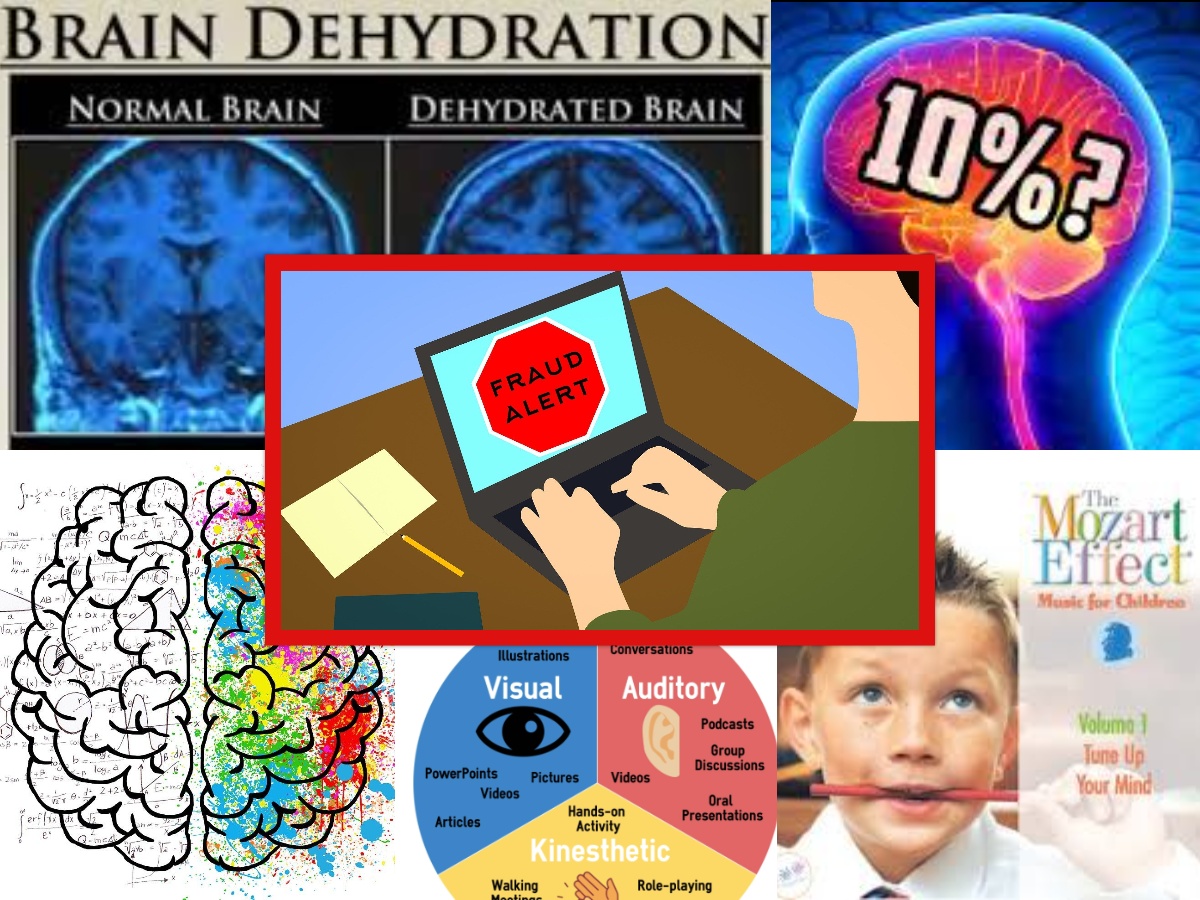
    Some of these ideas seem intuitive. Others, like the popular commercialized Brain Gym regimen which purports that rubbing areas of tissue around the sternum (called “brain buttons”) can help improve interhemispheric communication among other things, sound less feasible from the start (Hyatt, 2007). As quirky, benign, or even downright ridiculous as neuromyths can seem though, they are not harmless.  For every well-intentioned dollar and minute spent implementing policies based on pseudoscience, there are fewer resources left to give to evidence-based scientific principles. Like any opportunity-cost model, neuromyths “cost” a lot in terms of what we “could” be teaching and applying about the brain.” They also “cost” us in terms of public receptiveness and curiosity for new research. By simplifying complex topics and claiming knowledge we don’t actually have, neuromyths can give the impression that certain ideas are already “solved problems”,  when they are still questions we should be actively pursuing. In addition, when neuromyths are disproven, they may make people less trusting of true results from studies, since the previous “science” they heard wasn’t right. It lends substance to the notion that scientists are constantly “flip-flopping” on topics, hastily publishing results and then issuing retractions left and right, although the original claims were never made by scientists  in the first place. Allowing neuromyths to pass unchecked as truth undermines the credibility of neuroscience, and ultimately science as a whole, by propagating ill-informed ideas with the authority that the disguise of a “lab coat” gives the public.

    Given this context, it’s time to start challenging the beliefs we hold and start to critically differentiate between the “urban legends” of neuroscience and data-supported hypotheses. Try your hand at this quiz to see how well you know what is and is not true about the human brain and nervous system!

    TAKE THE QUIZ HERE: https://www.tryinteract.com/share/quiz/5f7fc0088a3cf300140577ed

    References:

    Bangarter, A., & Heath, C. (2004). The Mozart effect: Tracking the evolution of a scientific legend. British Journal of Social Psychology, 43, 605– 623.

    Boyd, R. (2008, February 07). Do People Only Use 10 Percent of Their Brains? Retrieved October 24, 2020, from https://www.scientificamerican.com/article/do-people-only-use-10-percent-of-their-brains/

    Craik, F. I., & Lockhart, R. S. (1972). Levels of processing: A framework for memory research3. Journal of Verbal Learning and Verbal Behavior, 11(6), 671-684. doi:10.1016/s0022-5371(72)80001-x

    Craik, F. I. M. & Tulving, E. (1975). Depth of processing and the retention of words in episodic memory. Journal of Experimental Psychology, 104(3), 268-294.

    Crockard, A. Confessions of a brain surgeon. New Scientist 2061, 68 (1996).

    Giuffre BA, Jeanmonod R. Anatomy, Sciatic Nerve. [Updated 2020 Jul 31]. In: StatPearls [Internet]. Treasure Island (FL): StatPearls Publishing; 2020 Jan-. Available from: https://www.ncbi.nlm.nih.gov/books/NBK482431/

    Draganski, B., & May, A. (2008). Training-induced structural changes in the adult human brain. Behavioural Brain Research, 192(1), 137-142. doi:https://doi.org/10.1016/j.bbr.2008.02.015

    Driemeyer J, Boyke J, Gaser C, Büchel C, May A (2008) Changes in Gray Matter Induced by Learning—Revisited. PLOS ONE 3(7): e2669. https://doi.org/10.1371/journal.pone.0002669

    Howard-Jones, P. Neuro, science and education: myths and messages. Nat Rev Neurosci 15, 817–824 (2014). https://doi.org/10.1038/nrn3817

    Hyatt, K. J. Brain Gym: building stronger brains or wishful thinking? Remedial Spec. Educ. 28, 117–124 (2007).

    Koch, C. (2016, January 01). Does Brain Size Matter? Retrieved October 16, 2020, from https://www.scientificamerican.com/article/does-brain-size-matter1/

    Lodish H, Berk A, Zipursky SL, et al. Molecular Cell Biology. 4th edition. New York: W. H. Freeman; 2000. Section 21.1, Overview of Neuron Structure and Function. Available from: https://www.ncbi.nlm.nih.gov/books/NBK21535/

    Macdonald, K., Germine, L., Anderson, A., Christodoulou, J., & McGrath, L. M. (2017). Dispelling the Myth: Training in Education or Neuroscience Decreases but Does Not Eliminate Beliefs in Neuromyths. Frontiers in Psychology, 8(1314). doi:10.3389/fpsyg.2017.01314

    Organisation for Economic Co-operation and Development. Understanding the Brain: Towards a New Learning Science. (OECD Publications, 2002).

    Pashler, H., McDaniel, M., Rohrer, D., and Bjork, R. (2008). Learning styles concepts and evidence. Psychol. Sci. Public Interest 9, 105–119. doi: 10.1111/j.1539-6053.2009.01038.x

    Pasquinelli, E. (2012), Neuromyths: Why Do They Exist and Persist?. Mind, Brain, and Education, 6: 89-96. doi:10.1111/j.1751-228X.2012.01141.x

    Nielsen, J. A., Zielinski, B. A., Ferguson, M. A., Lainhart, J. E., & Anderson, J. S. (2013). An evaluation of the left-brain vs. right-brain hypothesis with resting state functional connectivity magnetic resonance imaging. PloS one, 8(8), e71275.

    Rauscher, F., Shaw, G. & Ky, C. Music and spatial task performance. Nature 365, 611 (1993). https://doi.org/10.1038/365611a0

    Riener, C., and Willingham, D. (2010). The myth of learning styles. Change 42, 32–35. doi: 10.1080/00091383.2010.503139

    Ruigrok, A. N., Salimi-Khorshidi, G., Lai, M. C., Baron-Cohen, S., Lombardo, M. V., Tait, R. J., & Suckling, J. (2014). A meta-analysis of sex differences in human brain structure. Neuroscience and biobehavioral reviews, 39(100), 34–50. https://doi.org/10.1016/j.neubiorev.2013.12.004

    Treiman, R., Gordon, J., Boada, R., Peterson, R. L., and Pennington, B. F. (2014). Statistical learning, letter reversals, and reading. Sci. Stud. Reading 18, 383–394. doi: 10.1080/10888438.2013.873937

    Vellutino, F. R. (1979). Dyslexia: Theory and Research. Cambridge, MA: MIT Press.

    Wickelgren, W. (1981). Human learning and memory. Annu. Rev. Psychol. 32, 21–52. doi: 10.1146/annurev.ps.32.020181.000321

    Willingham, D. T., Hughes, E. M., and Dobolyi, D. G. (2015). The scientific status of learning styles theories. Teach. Psychol. 42, 266–271. doi: 10.1177/0098628315589505/;=   

    Wittbrodt MT, Millard-Stafford M. Dehydration Impairs Cognitive Performance: A Meta-analysis. Med Sci Sports Exerc. 2018 Nov;50(11):2360-2368. doi: 10.1249/MSS.0000000000001682. PMID: 29933347.

  • Milk’s environmental impact

    Milk’s environmental impact

         A big misconception is that milk is taken directly from a cow and put in a bottle.  But this is not entirely true as the process of turning raw milk into consumer milk is much more complicated than that. The process has an enormous environmental impact.  In recent years there has been a rise in popularity of plant-based milks because of its taste and health benefits, but are these new substitutes better for the environment?  The food sector has the highest consumption of water, and in fact, 86% of all the water in the world is used to grow food. The process of producing each type of milk generates their own water footprint.  A water footprint is an indicator of how much water both directly and indirectly is used by a customer or producer.  So you and I both have water footprints from eating food, driving our cars, taking showers, and many more things in our daily life.  The water footprint for milk is calculated by the total volume of freshwater that is, directly and indirectly, used to produce it.  The three main types of milk I am going to talk about will be cow milk, soy milk, and almond milk, and the water waste that is accumulated as part of the production process for these types of milk. 

         Growing up I always believed like many other people that milk came directly from a cow straight into the container.  But that is a huge misconception about the milk industry.  In reality, the milk needs to be processed multiple times before it can be packaged and shipped out.  Each year the milk industry generates 3.739 to 11.217 million m^3 of water waste. This amount of water is 1 to 3 times the volume of milk that is processed and packaged each year.  That means that for every 1L of cow milk 1,050L of water waste is generated.  Because of the lack of interest and knowledge in this topic from general people, many do not know the environmental impact that happens because of all the waste.  Some of this water waste accumulates during various systems of milk production in the factories, such as cleaning systems, cooling systems, and steam generators.  This cleaning system results in the clean water waste mixing with the cleaning solutions that are pumped through the unit.  This chemical mixture is still in the water when it is disposed of into the nearby river, land, and fields.  This chemical mixture is a highly odorous black sludge that can cause destructive environmental impacts.  

         Recently there has been a rise in the demand for milk alternatives that provide better health benefits.  Because of this, there has also been a rise in many misconceptions about the environmental impact of these alterations.  I know when I first learned about alternatives like soy milk and almond milk, I believed that while they had great health benefits they also had positive environmental benefits along with it.  While they do have the least water waste with the processing of the milk; other areas of the production process also accumulate water waste.  With all three milk substitutes, there is an increase in water waste from the crop production of these products.  For soy milk, every 1 L generates 297 L of water waste.  

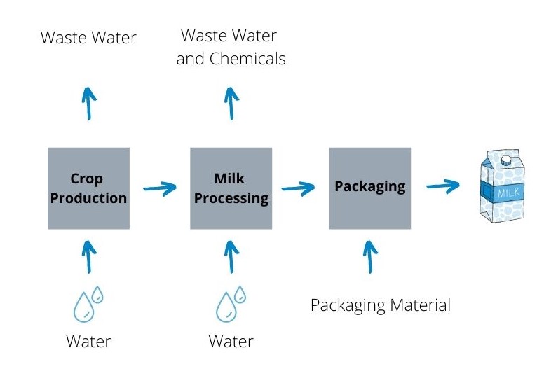
         Sadly out of the three milk options I looked at, there truly is no winner when it comes to lessening the environmental impact just based on picking a new milk substitute.  In the image, you can see the simplified engineering diagram for the production of milk.  In two of the stages for all types of milk, water is entering the system for crop production and the processing of milk.  While the amount of water that is used for each step is different depending on the milk, there still is an amount of wastewater that exists for each milk type.  But there are some ways production companies can adopt to decrease their water waste.  One way for almond milk would be to shift the sourcing and production of almonds to locations that have a more efficient irrigation system.  For cow milk, research might find a better way to streamline the process and to lessen the amount of chemicals introduced to water waste. 

    References: 

    Boguniewicz-Zablocka, J., Klosok-Bazan, I. & Naddeo, V. Water quality and resource management in the dairy industry. Environ Sci Pollut Res 26, 1208–1216 (2019). https://doi.org/10.1007/s11356-017-0608-8

    Courtney A. Grant and Andrea L. Hicks.Environmental Engineering Science.Nov 2018.1235-1247.http://doi.org/10.1089/ees.2018.0233

    Ercin, A., Aldaya, M., & Hoekstra, A. (2012, February 28). The water footprint of soy milk and soy burger and equivalent animal products. Retrieved October 08, 2020, from https://www.sciencedirect.com/science/article/abs/pii/S1470160X11004110?casa_token=e3EkrZ26r6IAAAAA%3Ad8BXC4T7XhPCDuL0uNN61qzA0XOht6XXqBIRrM1SH7_nN77SA7FbNk8jDSXLtqZUB29NnRasDXU

    Tikariha, A. , & Sahu, O. (2014). Study of Characteristics and Treatments of Dairy Industry Waste Water. Journal of Applied & Environmental Microbiology, 2(1), 16-22.