POV: you’re a college student who lives on her own. Not only do you have to do homework and go to class, but you also have to cook your own meals. While cleaning up after making your signature pasta dish (a spin-off of Gigi Hadid’s vodka pasta), you notice that your pan is really gross and grimy on the bottom. You scrub and scrub, but only a little if anything comes off. What can you do now? Enter: Bar Keepers Friend.
This cleaning agent comes in many different forms so that it can be used on many surfaces. Its creation is credited to a chemist named George William Hoffman who realized that cooking rhubarb cleaned up a tarnished pan of his. He ended up finding out the secret ingredient and sold a powdered version of it to his bar keeper friends to polish up any brass fixtures they may have. The secret ingredient? Lov– no it’s oxalic acid.
wikipedia.org
So when it comes to cleaning, there are different ways to do so: physically and chemically. As the description entails, physically cleaning something includes scrubbing, heat, light, and sound waves to clean a surface. With chemical cleaning, a reaction is used to remove dirt or anything from a surface. However, with chemical cleaning, some corrode surfaces more than others and are more toxic. Compared with other acids like hydrochloric acid and citric acid (which are both in-organic acids), oxalic acid is less corrosive. It can also complex with metal ions more effectively (aka can loosen up any built up schmutz and make it more dissolvable). But how does oxalic acid do that?
sciencedirect.com
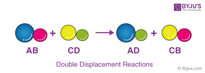
Let’s take rust for example. Rust (iron oxide) is oxidized iron and SUPER hard to get off of any pans or metallic surfaces. Don’t even get me started on how tough rust stains are on fabric and other woven stuff like rugs. When oxalic acid comes into contact with rust, it causes a double displacement reaction. What does that mean? The double displacement basically switches around the ions in the rust and oxalic acid, resulting in the rust to turn into iron oxalate. Iron oxalate is a salt that is water-soluble, allowing it to be washed away by water so TADAAA!!! We’ve cleaned our rusty pans and things.
byjus.com
Now, the brand, Bar Keepers Friend has expanded to more than just a powdered oxalic acid cleaner and takes many shapes and forms. You can use different products to clean stove tops, pans, and even your coffee machine. Of course, in order to be suitable for these places, they have to alter the formula. Their formula takes many forms, from liquids to powders to other liquids. For gentler surfaces, they’ve diluted the amount of oxalic acid. But at the end of the day, you could also just rub a piece of rhubarb on your pans and rust stains. After all, who said oxalic acid couldn’t be your friend too?
Resources:
Britannica, The Editors of Encyclopaedia. “oxalic acid”. Encyclopedia Britannica, 19 Dec. 2018, https://www.britannica.com/science/oxalic-acid. Accessed 20 November 2022.
He, Y. “Liquid-Based Microextraction Techniques for Environmental Analysis.” Comprehensive Sampling and Sample Preparation, Academic Press, 10 July 2012, https://www.sciencedirect.com/science/article/pii/B9780123813732001162#s0095.
Li, Yong-Sheng, et al. “Cleaning Effects of Oxalic Acid under Ultrasound to the Used Reverse Osmosis Membranes with an Online Cleaning and Monitoring System.” Desalination, Elsevier, 16 Apr. 2016, https://www.sciencedirect.com/science/article/pii/S0011916416301710.
“Our Story.” Bar Keepers Friend, 11 Feb. 2021, https://barkeepersfriend.com/about-us/our-story/?param1=value1¶m2=value2&keyword=barkeepers+friend&creative=595151622440&gclid=Cj0KCQiAveebBhD_ARIsAFaAvrGcdlz4IqwndBFsUDjLp0H5Hpi3VXFwBVovW5U7WUm76vXWCD3RraUaArjIEALw_wcB.
Renae. “Cleaning with Oxalic Acid? Here’s What You Need to Know.” CORECHEM Inc., 7 Sept. 2022, https://corecheminc.com/cleaning-with-oxalic-acid-heres-what-you-need-to-know/#:~:text=When%20Oxalic%20Acid%20comes%20in,water%20and%20easily%20rinses%20away.
The use of a system of differential equations to model the epidemiological dynamics of diseases across human populations has lately gained prominence. Several scholarly articles with SIR-type models of different infectious diseases have been developed (Tang et al. 2020). This has come to light in great part due to the global epidemics of Covid19 since early 2020. References to models from different researchers and institutions have anxiously focused on predicting the waves of cases, hospitalizations, and deaths. Questions like how, for example, isolation and quarantine would affect the dynamics of the disease were analyzed. Beyond the fear and concerns of the pandemic, the rise in prominence of these models have also extended into the public’s discourse. Otherwise obscure technical terms like “flattening the curve,” “herd immunity,” “reproduction rate”, “Ro,” among others, have become common terms used by the tv hosts, journalists, and people often without the correct interpretation or with lack of basic comprehension.
Concept Box 1. SIR refers to an infectious disease epidemiological model that at each point of time estimates the number of people from a given population who could be either susceptible to, S(t), infected with, I(t) or recovered from, R(t), an infectious disease; ergo its name is read S, I, R. Moreover, each letter in SIR is a differential equation that changes with time, t, and so the three equations form a system of differential equations, ergo the SIR model or SIR-type model.
Yet, researchers, epidemiologists and public health officers have been using SIR-type models to guide health policies for quite some time (Luz et al. 2010; Chowel et al. 2016; Opatowski et al. 2018). Specifically, these models have already been used for the design and evaluation of control and prevention strategies in respiratory diseases (Scherer et al. 2002; Smith et al. 2010). However, little is known by the layman about how these models work, what their strengths and limitations are, how useful they are for disease surveillance and how effectively they measure the effectiveness of control and prevention strategies. Without diving into technical concepts and features, this article aims to provide a brief description of these models as well as their strengths and limitations in the investigation and control of respiratory diseases.
A typical SIR model
Many names for a model: Various terms have been used to name these models and could cause confusion about whether one is referring to the same or different one. Among these terms are “Dynamic models,” “Mathematical epidemiology models,” “Compartmentalized models, “Disease transmission models,” “Transition dynamic models,” “Group-structured epidemic models,” etc. In general, it could be said that these models are at the same time dynamic, mathematical, compartmentalized and describe disease transmission through rates of transitions among compartments (Chowell et al. 2016). Each one of these terms could well be used to describe these models.
However, the term that has gained more traction is SIR-type models for how the name describes the structure of the models. We will use this term along this article under the understanding that we are referring to the other terms as well.
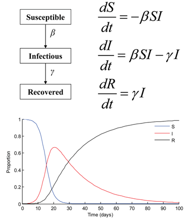
Structured SIR model: Among these models, the one with the simplest structure is the SIR model. Precisely, SIR stands for Susceptible, Infected and Recovered compartments (Figure 1). The names of these compartments are describing the health status of a fraction of a given population, when considering a specific infectious disease (Tang et al. 2020). Specifically, given an infectious disease, at a point of time a fraction of the population is susceptible, another fraction is infected and another one recovered, making the sum of the three compartments up to the total population size, N, namely, S + I + R = N. Namely, these compartments describe mutually exclusive groups of individuals.
Figure 1: Typical SIR model: the compartments, differential equations and progression of population disease states for susceptible, infected, and recovered compartments.
At an individual level, it could be said that the health status of a person is either susceptible, infected or recovered; namely a person’s health could not be in two compartments at the same time. Now, the transmission or the dynamics feature happens in intervals of time; namely, in an SIR model it is through time how parts of a population (or the probability that an individual) transitions from being susceptible to being infected and then to being recovered. In this example presented in Figure 1, the entire population becomes infected and eventually recovers.
Concept box 2. Each step along S, I or R disease status and transitions follows a specific rate in time: an infection rate that depends on the effective interaction between susceptible and infected individuals, , from susceptible to infection and a recovery rate, , from infected to recovered (Tang et al. 2020). A system of three differential equations with S, I and R as time-dependent variables and with transition rates as function parameters could be built along with initial conditions and balances.
Incrementally complex models
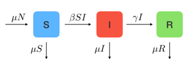
The model in Figure 1 is the simplest SIR model and helps only to illustrate the disease dynamics. Two additional components: the birth rate and the mortality rate provide more practical use. SIR models often assume a birth rate that increases the size of the population and usually it is an addition to the “Susceptible” compartment, meaning that all new births are susceptible to the specific infection disease. SIR model also distinguishes two types of mortality rates: one caused by factors other than the specific infectious diseases in the model, , and the second is the rate of death explicitly attributable to the infectious diseases being modeled, .
Figure 2: Typical SIR model with birth, non-disease and diseased-caused mortality rate. N stands for the total population, b for birth rate, , for all other causes mortality rate and , for infection-caused mortality rate.
However, adding mortality to SIR models is just one thin layer in the many other more complex configurations. SIR models become incrementally more complex in different ways depending on how the infectious disease behaves in the population. These variations are called SIR-type models. Among the many factors determining the model configuration, three are the most frequently observed: clinical course of the disease, demographic-driven modifications, and different disease risk conditions among groups in the population (Purkayastha et al. 2021).
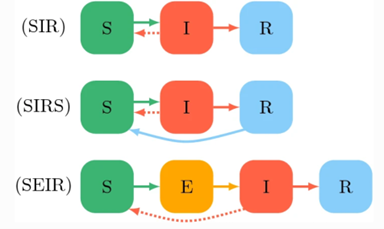
Figure 3: Incrementally complex SIR models with modifications due to waning of protection after recovered from infection (SIRS) or when a susceptible individuals become exposed as an intermediate stage before confirming infection (SEIR)
Among SIR configurations based on the clinical course of the disease is, for example, the SIRS models (Figure 3, mid-section). In general, this configuration is used to capture how the immunity gained by those who recover from infections wanes in time and, thus, makes them susceptible to reinfection (blue arrow from R to S). This clinical feature has also and often been observed in respiratory diseases when new variants of the pathogen causing the disease mutates significantly as in the annual influenza epidemics or as in the variant-driven waves in Covid19.
By the same token, a SEIR configuration (Figure 3, bottom) is used to model diseases like Covid19 when susceptible individuals are exposed to the pathogen causing the disease, but due to the clinical course of the infection (i.e., duration of the incubation period) or due to individual characteristics such as immunological conditions, may potentially result as infected or not. Also, when information about being exposed is known and individuals modify their behavior, i.e., self-isolation, until the infection diagnosis is confirmed or rejected.
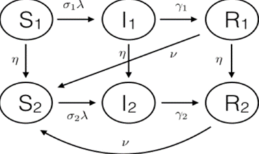
One of the most frequent demographic-driven modifications is the age-structured SIR model (Figure 4). The main reason for an age-structured SIR model is the differential behavior of infection (or course of the disease) and impact across age groups. This feature implies, among other characteristics, that different rates for each age group of either infection, recovery, or disease-caused mortality rates (or rates of other outcomes such as hospitalization) could be attributable to the same pathogen (Brand et al. 2020). Moreover, the interaction between different age groups could produce differences in the probability of transmission and infection. Facts like these have been observed in seasonal influenza as well as in Covid19 when the transmission and mortality seem to be different for different age groups. As shown in Figure 4, the SIR model includes two sets of S, I and R compartments, each subscript representing the specific population fraction of susceptible, infected and recovered of age group 1 and 2, respectively.
Figure 4: Basic age-and-disease state compartmental model with disease transitions, aging transitions and waning of immunity protection.
Concept Box 3. Two additional elements: First, is the transition probabilities or rates are specific to each age group and that aging is also represented by the transitions between compartments of susceptible as well as between infected and recovered across age groups. Second, similar to the SIRS model mentioned above, the figure also shows waning of immunity when those who recover from infection become susceptible again to reinfection.
Regarding modifications to the SIR model due to risk conditions among groups in the population, it is possible to have a structure similar to the described in Figure 4. Specifically, instead of age groups, there could be risk groups such as “high risk” for infection and severe outcomes (i.e., immunocompromised) versus non-high risks (i.e., immunocompetent) (Thomas et al 2020). Diseases like influenza and now Covid19 have shown different risks of severe outcomes given infection, like having comorbidities or immunocompromised conditions (Brand et al 2020). Figure 4 could also represent disease differences (i.e., different rates of incidence, prevalence) in the group of healthcare workers versus the general population (Thomas et al 2020).
It should be noted that the systems of differential equations representing the models described in Figures 2, 3 and 4 would incrementally be more complex than the system represented in Figure 1. Specifically, the structure of the three equations in Figure 1 would dramatically change (Chowel et al. 2016, Tang et al. 2020). Moreover, the number of differential equations will increase with the number of compartments modeled and the number of parameters such as the transition rates would also increase proportionally.
Reproductive number and Herd immunity
Perhaps the two most important epidemiology concepts in SIR models are the average reproductive number and the herd immunity threshold. The two concepts are specific to each disease and pathogen.
Concept Box 4. Herd immunity. This concept refers to the minimum percentage of people within a community who need to be immune to an infectious disease in order to reduce the size of the outbreak leading to its disappearance (Law et al. 2021; Royal Society 2020). Alternatively, it could be thought of as the minimum percentage of people needed to be immune to prevent an increasing outbreak. Immunity can occur from either a prior infection or from vaccination.
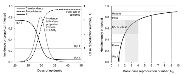
Figure 5a shows how the herd immunity is achieved when the proportion of those recovered levels out in time. While Figure 5b shows the relationship between herd immunity and reproductive number.
Figure 5: a) Build-up of herd immunity during a model epidemic of SARS CoV-2. b) Herd immunity threshold in relation to Ro, comparing SARS CoV-2 with influenza A, Ebola virus disease, Poliomyelitis and Rubella.
Concept Box 5. Basic reproductive number: The average reproductive number (Ro, pronounced R-nought) is the number of secondary infected cases caused by a single case during the course of the illness in a susceptible population. In simple words, how many new cases would appear for every single infected case is what Ro measures. In the first SIR model (Figure 1), Ro would be calculated as the ratio between β and γ. Naturally, in successive models the mathematical expression for Ro would have to be modified accordingly but would preserve the intuitive definition.
It is known, for example, that measles has a reproductive number of 14.5 (with Ro ranging from 13 to 16), which means that each case of measles could on average infect approximately 14 susceptible persons (Royal Society 2020). On the other hand, influenza and Covid19 have an Ro equal to 1.6 (range 1 to 3) and 2.6 (range 2 to 4), respectively. The key message here is that, when Ro < 1, the disease will eventually perish in the population, and if Ro > 1, the disease will keep spreading faster, the greater this number is.
Although not in a linear fashion, the basic reproductive number and the herd immunity threshold have an inverse relation between them; namely, when the percentage of people in a population immune to an infectious disease increases, the chance for secondary infections decreases substantially. This is seen by the following expression Herd Immunity = 1 + (1/Ro) x 100. In it, we see that the herd immunity threshold is inversely related to the basic reproductive number (Figure 5b). Specifically, when the force of infection substantially decreases down to a point where Ro < 1, (Figure 5a), the disease will perish in the population mainly because the percentage of people immune to the disease is high enough to provide protection to the rest of the remaining susceptible in the population, e.g., indirect protection, which is referred as “herd immunity.”
Using SIR models: control and prevention
Designing a SIR model is further from being just an academic or theoretical exercise. The dynamic features of SIR-type models have been used not only to elegantly describe the epidemiological progression of an infectious disease outbreak in a population, but also to predict its future health burden and progression (Tolles et al. 2020, Xu et al. 2021). They have been used to design practical and effective strategies that reduce the disease burden. Specifically, a SIR model, when properly designed, would be able to measure and predict the health impact of the infectious disease in absence of an intervention (i.e., the model could estimate the number of disease cases, associated hospitalization or deaths) as well as measuring the potential impact of disease control and prevention strategies. In other words, the effectiveness of an intervention would be assessed by the relative or proportional reduction in the disease impact compared to the absence of intervention (i.e., relative or proportional reduction in disease cases, associated hospitalizations or deaths).
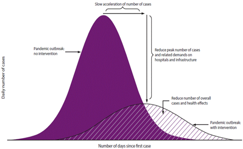
Concept box 6. Flattening the curve: At the beginning of the Covid19 pandemic and for months, the “flattening the curve” expression was often heard, mostly as a question, “how to flatten the curve?” Any strategy addressed to control or prevent a disease outbreak or a large epidemic such as the Covid19 could be considered a “flattening the curve” strategy (Figure 6); namely, strategies that leads to the deceleration in the number of cases causing a reduction in their daily and overall numbers during the pandemic (Specktor 2020).
Figure 6: Flattening the curve refers to those strategies that decrease the effective contact rate, β, that also decreases Ro, delaying and lowering the peak of daily infection rate that occurs in an epidemic. The figure measures the epidemic curve of the daily number of cases, but it could also measure hospitalizations or deaths.
During a large outbreak that overwhelms the healthcare system in a given population, flattening the curve below the healthcare system capacity would prevent its collapse. This becomes crucial when the number of hospital beds, respiratory devices or other resources are limited and when there are no prophylactic methods available such as vaccines, antivirals or antibacterials that could be used to prevent the infections among susceptibles or cure the disease among infected. In the early months of the Covid19 pandemic, social distancing of susceptibles along with wearing masks and hand washing were promoted to reduce the daily number of cases. When exposures happened and infection was suspected, isolation and quarantine were also recommended (Xu et al. 2021). All these non-pharmaceutical-based recommendations sought to decrease and maintain low social interactions within the communities and, by doing so, reduce disease transmission, seeking a low β, which eventually would decrease Ro (Figure 6).
Social distancing: In general, keeping the daily number of disease cases at a manageable level for healthcare providers to be able to provide medical services was desired to be sustainable in time. However, we have seen how healthcare capacity in some places and times was overwhelmed by the high level of new daily cases. In SIR models, social distancing has been introduced following different approaches and could help to visualize where these increases in healthcare demand would happen.
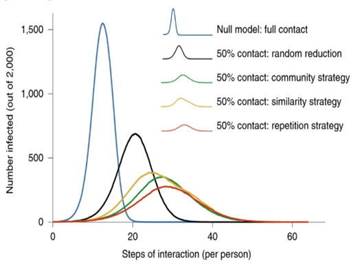
In SIR models, the effectiveness of “flattening the curve” of different contact reduction strategies could have a different impact when compared to no social distancing, i.e., full contact (Figure 7). As we can observe, it is not only the reduction in the frequency of contacts (i.e. 50% reduction in contacts), but also whether the contact is random with any member in the community or repetitive with a selective group in the population (Block et al. 2020). Each type of interaction could significantly affect the shape, size and peak of the flattened curve.
Figure 7: The effectiveness of “flattening the curve” of four different contact reduction strategies when compared to no social distancing (i.e., full contact). Two determinant factors are the reduction in the frequency of contacts and how the contact takes place.
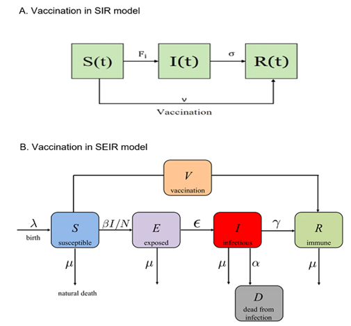
Concept Box 7. Vaccination in SIR models: When available, the most effective strategy to prevent large epidemics of infectious diseases is the use of vaccines. However, vaccines for new and emergent diseases that cause large outbreaks are often unavailable at the beginning of the epidemics. SIR models of infectious diseases can include vaccination strategies and then be able to predict the effectiveness impact of vaccination programs (Scherer et al 2002).
Figures 8a and 8b show the impact of vaccination by either including a rate of vaccination from susceptible individuals to recovered (the SIR model with vaccination rate v, Figure 8a) or by including a new compartment, vaccinated individuals, V, which is different that those recovered (Figure 8b). In both cases, susceptible avoid being infected by being vaccinated.
Figure 8: Modeling vaccination strategies in SIR-type models: (a) in classical SIR model and (b) in SEIR model as in Covid19.
Take-away message
A SIR model as any mathematical model is a simplification of how the infectious disease behaves in the population. It is suppose to capture the essential elements of a natural phenomenon: the dynamics of an infectious disease in the population. When well designed and calibrated, it could be a reliable tool, a working hypothesis that helps in the prediction, control and management of the disease impact. However, SIR-type models depend on their assumptions and on the data fed to the model (Adamu et al. 2019). The assumptions are usually educated guesses about many key clinical, epidemiological, and demographic components in the model for which robust data are not available. The assumptions are made to solve part of the uncertainty about such components. Assumptions, for example, about how transmission happens in the community versus in healthcare settings or close environments, our assumptions about how a new treatment works or how long the vaccine protection lasts would change the outcomes of the model. When high quality data are available, the model would depend less on assumptions and more on evidence provided by the data (Tang et al. 2020).
It should be noted that if there were enough high-quality data for all key epidemiological components, one could just statistically analyze these data to then guide recommendations (Xu et al. 2021). That would make SIR models less necessary or even irrelevant. However, perfect information is seldom the case in sudden large epidemics of new diseases and so, SIR modeling helps to integrate the scarce data available with well-educated assumptions about those areas where uncertainty remains. In this context, the SIR models could be seen as a state of knowledge in between two learning scenarios: the complete uncertainty where everything is ignored and the full availability of data about the disease in the population (Tolles et al. 2020). In that sense, SIR modeling uses what is known and what is assumed about the disease and its burden to calibrate the model parameters and then see if the dynamics of the model replicates the reality of the disease. Various statistical, numerical and approximation approaches could be used to calibrate the SIR models.
Additionally, one could suspect that there is a minimum of data needed to design a useful SIR model. Among them disease-, country- and region- specific epidemiological data would be required. Also, disease-specific clinical data regarding the outcomes of infections; namely, proportion of infected people fully recovered, recovered with temporary or permanent sequelae or portions of infected who die (Chowell et al. 2016). Along these lines, the specific effectiveness of available treatments, of control strategies like wearing masks, washing hands, or social distancing would also be helpful. Population data such as size of risk groups or age groups would be important when the disease impact is different depending on the risk, age or comorbidity conditions of some groups in the population (Brand et al. 2020).
Overall, SIR-type models of infectious diseases have become important tools. Researchers, biologists, epidemiologists, and public health officers who are focused on predicting, controlling and preventing the impact of large outbreaks or epidemics caused by emerging infectious diseases resort to these models. This article aimed to introduce in no-technical terms the main characteristics and virtues of these models. I do understand that these notes are quite incomplete and only cover a few topics among many related others without going into the complexities. However, the aim is to provide an informal introduction to these models and how useful they could be when dealing with population health events in the future
References:
Adamu HA, Muhammad M, Jingi AM, Usman MA. Mathematical modeling using improved SIR model with more realistic assumptions. International Journal of Engineering and Applied Sciences (IJEAS). 2019. 6. 10.31873/IJEAS.6.1.22.
Block P, Hoffman M, Raabe IJ. et al. Social network-based distancing strategies to flatten the COVID-19 curve in a post-lockdown world. Nat Hum Behav 4, 588–596 (2020). https://doi.org/10.1038/s41562-020-0898-6
Brand SP, Munywoki P, Walumbe D, Keeling MJ, Nokes DJ. Reducing respiratory syncytial virus (RSV) hospitalization in a lower-income country by vaccinating mothers-to-be and their households. Elife. 2020 Mar 27;9:e47003. doi: 10.7554/eLife.47003. PMID: 32216871; PMCID: PMC7556875
Chowell G, Sattenspiel L, Bansal S, Viboud C. Mathematical models to characterize early epidemic growth: A review. Phys Life Rev. 2016;18:66-97. doi:10.1016/j.plrev.2016.07.005 https://www.ncbi.nlm.nih.gov/pmc/articles/PMC5348083/
Law KB, M Peariasamy K, Mohd Ibrahim H, Abdullah NH. Modelling infectious diseases with herd immunity in a randomly mixed population. Sci Rep. 2021;11(1):20574. Published 2021 Oct 18. doi:10.1038/s41598-021-00013-2 https://www.ncbi.nlm.nih.gov/pmc/articles/PMC8523531/
Luz PM, Struchiner CJ, Galvani AP. Modeling transmission dynamics and control of vector-borne neglected tropical diseases. PLoS neglected tropical diseases, 2010 4(10), e761. https://doi.org/10.1371/journal.pntd.0000761
Opatowski L, Baguelin M, Eggo RM. Influenza interaction with cocirculating pathogens and its impact on surveillance, pathogenesis, and epidemic profile: A key role for mathematical modeling. PLoS Pathog. 2018;14(2):e1006770. Published 2018 Feb 15. doi:10.1371/journal.ppat.1006770 https://www.ncbi.nlm.nih.gov/pmc/articles/PMC5814058/
Purkayastha S, Bhattacharyya R, Bhaduri R. et al. A comparison of five epidemiological models for transmission of SARS-CoV-2 in India. BMC Infect Dis 21, 533 (2021). https://doi.org/10.1186/s12879-021-06077-9
Scherer A, McLean A. Mathematical models of vaccination, British Medical Bulletin, Volume 62, Issue 1, July 2002, Pages 187–199, https://doi.org/10.1093/bmb/62.1.187
Smith AM, Ribeiro RM.Modeling the viral dynamics of influenza A virus infection. Crit Rev Immunol. 2010;30(3):291-8. doi: 10.1615/critrevimmunol.v30.i3.60. PMID: 20370636 https://www.dl.begellhouse.com/journals/2ff21abf44b19838,1629d2c3507c27c5,5aa3a295481caaac.html
Specktor, B. (2020, March 16). Coronavirus: What is ‘flattening the curve,’ and will it work? LiveScience. Retrieved April 18, 2022, from https://www.livescience.com/coronavirus-flatten-the-curve.html
Tang L, Zhou Y, Wang L, Purkayastha S, et al. A Review of Multi-Compartment Infectious Disease Models. International Statistical Review, Volume88, Issue2. August 2020. Pages 462-513 https://onlinelibrary.wiley.com/doi/10.1111/insr.12402
The Royal Society. Herd immunity in the epidemiology and control of COVID-19. SET-C-Rapid Review, November 26, 2020. Available at https://royalsociety.org/-/media/policy/projects/set-c/set-c-herd-immunity.pdf
Thomas DM, Rodney S, Nikhil V D; Swati D, Nicholas C. A Primer on COVID-19 Mathematical Models. Obesity Vol. 28, Iss. 8, (Aug 2020): 1375-1377
Tolles J, Luong T. Modeling Epidemics With Compartmental Models. JAMA. 2020; 323(24):2515–2516. doi:10.1001/jama.2020.8420
Xu Z, Wu B, Topcu U. Control strategies for COVID-19 epidemic with vaccination, shield immunity and quarantine: A metric temporal logic approach. PLoS One. 2021 Mar 5;16(3):e0247660. doi: 10.1371/journal.pone.0247660. PMID: 33667241; PMCID: PMC7935317. https://journals.plos.org/plosone/article?id=10.1371/journal.pone.0247660
Specific references from where Figures 1 to 8 were borrowed for this article
For Figure 1.
Luz PM, Struchiner CJ, Galvani AP. Modeling transmission dynamics and control of vector-borne neglected tropical diseases. PLoS neglected tropical diseases, 2010 4(10), e761. https://doi.org/10.1371/journal.pntd.0000761
For Figure 2.
Sasaki, K. (2020, March 11). Covid-19 dynamics with sir model. The First Cry of Atom. Retrieved April 20, 2022, from https://www.lewuathe.com/covid-19-dynamics-with-sir-model.html
For Figure 3:
Dias S, Queiroz K, Araujo A. Introduction to Group-Structured-Epidemic Model. J Control Autom Electr Syst 33, 23–37 (2022). https://doi.org/10.1007/s40313-021-00841-7 https://link.springer.com/article/10.1007/s40313-021-00841-7
For Figure 4:
Brand SP, Munywoki P, Walumbe D, Keeling MJ, Nokes DJ. Reducing respiratory syncytial virus (RSV) hospitalization in a lower-income country by vaccinating mothers-to-be and their households. Elife. 2020 Mar 27;9:e47003. doi: 10.7554/eLife.47003. PMID: 32216871; PMCID: PMC7556875
For Figure 5:
The Royal Society. Herd immunity in the epidemiology and control of COVID-19. SET-C-Rapid Review, November 26, 2020. Available at https://royalsociety.org/-/media/policy/projects/set-c/set-c-herd-immunity.pdf
For Figure 6:
Specktor, B. (2020, March 16). Coronavirus: What is ‘flattening the curve,’ and will it work? LiveScience. Retrieved April 18, 2022, from https://www.livescience.com/coronavirus-flatten-the-curve.html
For Figure 7:
Block P, Hoffman M, Raabe IJ. et al. Social network-based distancing strategies to flatten the COVID-19 curve in a post-lockdown world. Nat Hum Behav 4, 588–596 (2020). https://doi.org/10.1038/s41562-020-0898-6
For Figure 8: (two references)
Law, K.B., M. Peariasamy, K., Mohd Ibrahim, H. et al. Modeling infectious diseases with herd immunity in a randomly mixed population. Sci Rep 11, 20574 (2021). https://doi.org/10.1038/s41598-021-00013-2
Xu Z, Wu B, Topcu U. Control strategies for COVID-19 epidemic with vaccination, shield immunity and quarantine: A metric temporal logic approach. PLoS One. 2021 Mar 5;16(3):e0247660. doi: 10.1371/journal.pone.0247660. PMID: 33667241; PMCID: PMC7935317. https://journals.plos.org/plosone/article?id=10.1371/journal.pone.0247660
The global warming clock says we have 15 years left before we reach a temperature point of no return. Will I be alive by the time I’d be 40? I want to grow up and live a full life. I want a career, a husband, and kids of my own. Will our planet continue to be viable by then? Am I ever going to get the future I want? Oh god, I need to do something. What could I possibly do to prevent the death of my home?
Looking back now, Action has always been my go-to weapon. I despise feeling helpless. Author and Holocaust survivor Elie Wiesel once said, “The opposite of love is not hate, it’s indifference.” His words have become my mantra as I continue to address the indifference we as a human race are posing on Earth: Pollution. More specifically, plastic pollution.
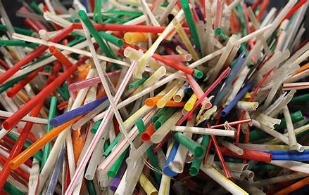
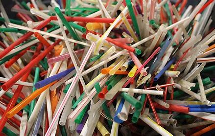
While plastic in general is an important predicament in the race to save Earth, most of it can be and is being recycled. However, It’s a specific use given to plastic that appears to be causing trouble. Plastic straws. I remember the first time I heard about the ban on plastic straws, and how absurd it sounded at the time. Plastic straws? Couldn’t they simply be recycled? Evidently, no. Recycling facilities don’t take them because their small size is a risk to the function of the big machines, as they often fall into the cracks. As I had predicted, the number of plastic straws produced and distributed barely decreased after the straw ban. They’re too practical to get rid of so hastily. This was not enough for me. If my planet, my home was dying, then something had to be done.
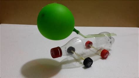
For a long time, I continued to ask myself how I can reuse, and possibly, improve the use of these dilapidated pieces of plastic. It wasn’t until my father suggested I teach myself some basic programming to build robots, such as an RC car that the idea seemed to be right there, screaming right in my face. Yes, learning how to program was a great idea, but using that programming to think outside of the box became the goal. I wanted, no, needed to find a way to help this worldwide dilemma; my desire for Action had to be fulfilled. While a single plastic straw may seem insignificant, it’s the billions of straws that truly impact the environment. Using some of my creativity, I decided I was going to build a remote control car made out of plastic straws.
After extensive research, I learned everything I needed to build my prototype. Due to my lack of knowledge in the field of computer programming, I commenced my project by making one with only an on-and-off switch. I melted my straws using nothing but some baking paper and a clothes iron, hot glued all of my melted pieces together and built my very first straw car. It was a start, and I hoped to eventually make the car durable and physically appealing enough for a child to play with. But this is only the beginning.
Making a more durable car starts by transforming the straws into a more durable material. Straws are made out of polypropylene which warps easily. Suppose I could learn to blend polymers effectively and convert polypropylene into a stronger material. In that case, the straws’ plastic could be repurposed into infinite recycled possibilities–much like my car. Our ancestors have always wanted a better future for the following generations, and we should want the same for our descendants.
If you’re even tangentially related to the tech world, you’ve probably heard an awful lot about Quantum Computing recently. But what exactly is it? Why is it useful? What is the point? And what does it mean for the future of computers for everyday people like you and me?
What is Quantum Computing?
The basic idea behind quantum computing is that rather than having binary 1’s and 0 build the computer, you have a range of values between 0 and 1, determined by the superposition and entanglement of subatomic particles in the computer. Now this may sound scary, but it’s actually quite similar to what’s going on in your normal computer. The 1’s and 0’s you always hear about making up binary are actually just electrons. Electrons either flow through transistors (producing a 1) or they don’t (0). Computers have always relied on sub-atomic particles, we’re just changing which ones we rely on with quantum computing.
Quantum computers were proposed in the 1980s by Richard Feynman and Yuri Manin. But it wasn’t until 1998 that Isaac Chuang at Massachusetts Institute of Technology (MIT) and Mark Kubinec of the University of California at Berkeley created the first quantum computer (2-qubit) that could be loaded with data and output a solution. These computers have been theorized for a long time, but only recently are starting to become viable tools.
What does that mean for me?
Now, before we continue, I want to be clear that in the next 10-20 years, consumers will not be using quantum computing in their homes. There are a lot of advantages we’ve found to using the range of values that quantum provides, but those advantages are not currently applicable to daily users checking emails or watching videos; what they are good for is searching databases.
What is Quantum Computing useful for, then?
Binary-based computers are particularly bad at searching for values. In fact, most search algorithms are just special tricks to get around how bad computers are at finding values in a dataset. This is because binary values have to check each value they come across one at a time and “label” each one as not the object they’re looking for. What quantum computing allows is, rather than going one-by-one, searching all (or many of the) values at the same time.
In a similar vein, quantum computing is quite good at modeling possible outcomes of situations because rather than having to cycle through each scenario one at a time – like a binary computer – it can process many different models at once. These advancements will be massive for many areas of scientific study by exponentially decreasing the amount of time/resources computing models takes.
Closing thoughts
If you are an average consumer like me, these advancements won’t affect you directly for many years, but I estimate we will be seeing faster scientific breakthroughs in coming years as computing time continues to decrease.
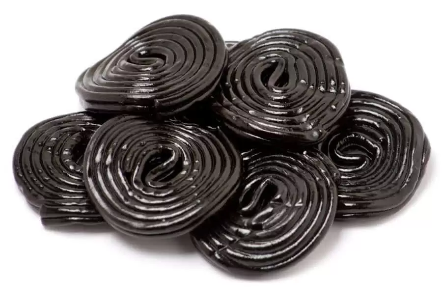
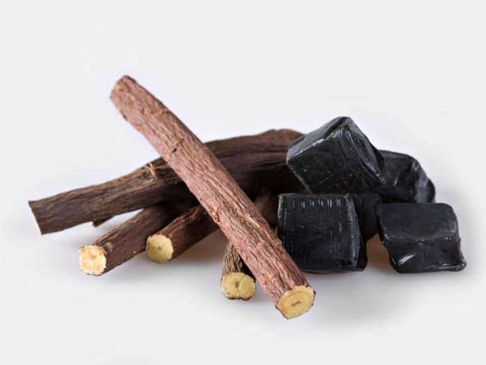
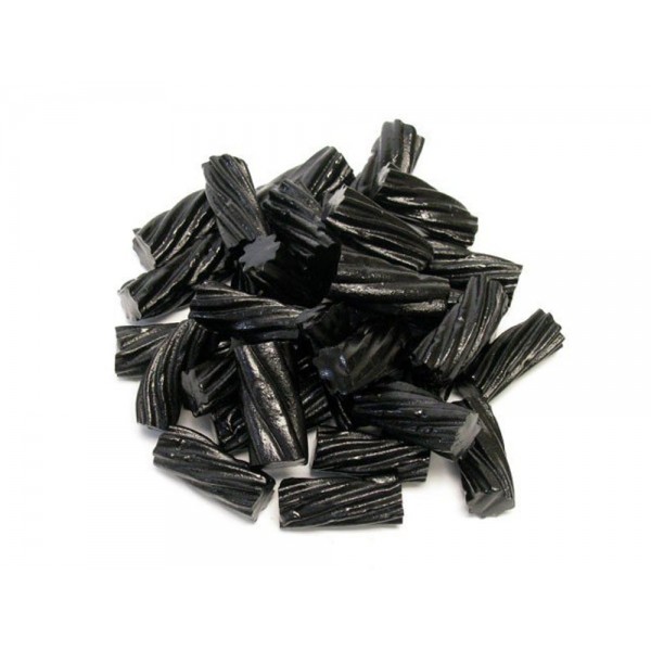
Black licorice. You either love it or you hate it. Some delight in the intense spice flavor that comes with a bite of licorice and others find it repulsive and gag at the mere scent of it. As a divisive food and old-timey treat, black licorice has a long history of being a chewy confectionery and a popular flavor for drinks and tobacco in many parts of the globe. Licorice (scientifically referred to as Glycyrrhiza glabra) is a flowering plant that comes from the legume family. Its roots contain the flavor that we know as licorice and are commonly extracted for various uses. While it shares similar flavoring compounds, it is not related botanically to anise or fennel as some may think. (though sometimes they are used instead of licorice to evoke the same flavor profile)
What makes black licorice so sweet?
The iconic scent and flavor of licorice come from a mix of different compounds, but the one that gives it most of its sweetness is glycyrrhizin (a compound that is about 50 times sweeter than sugar!) This sweetness is different than regular sugar in that it more closely resembles sweeteners like Sweet ‘n’ Low which is comprised of saccharin. Some people vehemently dislike this type of sweetness which is also known to linger on the tastebuds for longer. Many people claim to dislike how “sickeningly sweet” it is and feel that it strongly dominates whatever you taste in your mouth for many minutes even after it is consumed. Others say that their aversion comes from the glycyrrhizin tasting more bitter than sweet.
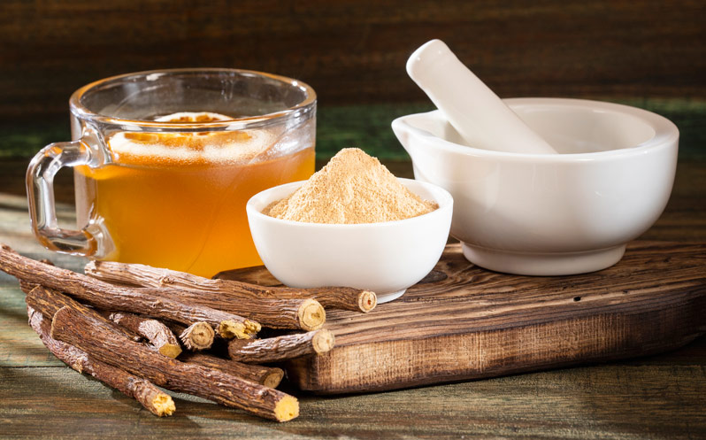
This bitterness can be attributed to herbal medicine, which licorice is also known to be useful for. There are many patented licorice-based medicines in China, where its extract is used in the treatment of bronchitis, colds, cough, and upper respiratory diseases. Glycyrrhizin, glycyrrhizinic acid, isoliquiritin, and glycyrrhizic acid are the most notable substances used for health benefits as they possess anti-cancer, anti-microbial, and anti-inflammatory properties. Excessive consumption that allows for the build-up of these compounds, however, may lead to serious adverse health effects.
Consequences of Overconsumption
Like most things in life, licorice is best enjoyed in moderation, but for more sinister reasons than you may think. Eating more than 57g of black licorice a day for at least 2 weeks could potentially cause serious health problems, such as an increase in blood pressure and an irregular heart rhythm (arrhythmia). This happens because of an excess of glycyrrhizic acid in the body. Normally your body is able to process glycyrrhizic acid into glycyrrhetinic acid, which is relatively harmless in small amounts, but when larger concentrations are present in the body, it can inhibit an enzyme that assists in converting active cortisol (the hormone that controls adrenaline) into inactive cortisone. You can imagine what too much active cortisol might do to your body, and this imbalance like this can wreak havoc on your body.
Cortisol is a hormone that plays a role in your fight-or-flight response and is similar chemically and structurally to aldosterone, which during a stressful event can signal to the body to hold on to water if you’re dehydrated. It does this by binding to structures in the kidneys that cause sodium to be pulled from urine in order to trigger osmosis and cause water to stay in your cells. Sodium has a +1 charge, however, and if it’s taken from the urine, then another +1 charge must replace it. This is done by potassium which can then replace the sodium in the urine and be excreted from the body. Now, when cortisol is present in concentrations that are dangerously high, it can be concluded that it would cause your body to pull more sodium from your urine, and you would lose more potassium right?
Cortisol (left) & Aldosterone (right)
This leads to hypokalemia or low potassium presence in blood, which can be detrimental to the muscles of your body especially one of your most essential muscles, your heart. Potassium is an ion in your body that signals a relaxation of your muscles after a contraction. If there isn’t enough potassium present in your blood, then your muscles will stay contracted, which can be especially bad for your blood vessels and your heart. This is where the increased blood pressure and arrhythmia can restrict proper oxygen flow throughout your body and cause your organs to shut down.
No Need to Panic
Now, of course, the chances of this happening to the average black licorice fan are very slim as long as the treat is enjoyed in moderation. Since most people wouldn’t eat 57g of black licorice every day, I think it’s safe to say that fearing death by licorice overdose won’t be found in anyone’s nightmares. All in all, black licorice is a novel sweet with an interesting chemical makeup that is loved (or hated) by many across the globe.
Wahab S, Annadurai S, Abullais SS, Das G, Ahmad W, Ahmad MF, Kandasamy G, Vasudevan R, Ali MS, Amir M. Glycyrrhiza glabra (Licorice): A Comprehensive Review on Its Phytochemistry, Biological Activities, Clinical Evidence and Toxicology. Plants (Basel). 2021 Dec 14;10(12):2751. doi: 10.3390/plants10122751. PMID: 34961221; PMCID: PMC8703329.
Within the past 200,000 years, modern humans began to appear. Though it took thousands of years to get to the Industrial Revolution, since then, technology has grown exponentially. In fact, the majority of new breakthroughs in technology have occurred within the past 250 years. Compared to the span of human existence, this time period is fractional, and it goes to show the rapid changes made in the technology sector.
In 1942, the first modern digital computer was built, and it weighed over 700 pounds. This machine was called the Atanasoff–Berry computer, or ABC. This machine was built to compute calculations with up to 29 variables, and it performed one operation every 15 seconds. Fast forward only 80 years to 2022, when Apple released their new Macbook Air. This laptop barely weighs 3 pounds and can perform millions of computations per second. It has a 1080p camera and has configurable storage up to 2T. Not even at 1% of the weight of the ABC, the Macbook Air can do so much more, and only within 80 years of development too. What the ABC could do then, the Apple Watch can do now. The progress has been extremely rapid in the last few years, and that leads me to stop and wonder: Will we hit a roadblock soon? Will there be no more changes left to make? What’s next in the future of technology?
Every couple of years, humans make incredible progress in the technological world. In the last 2,000 years, technology has advanced exponentially. When we imagine the future, we think of robots, advanced technologies, and even a cyberpunk-esque environment. The 1985 classic film, Back to the Future, got a lot right about modern technology, but it was also quite ambitious with some predictions. For example, the flying car, hoverboard, and the sleep-inducing alpha rhythm generator are all inventions that don’t exist today. On the other hand, the power lacing shoes, drones, and biometric devices are examples of technology that do exist now. Now while some of these technologies might never exist, one can’t help but wonder, which ones will? In the 20th century, the idea of the future was very metallic, robotic, and monochromatic. Now when we imagine the future, we imagine AI, big cities, and advanced tech in every aspect of our lives. So what does the future hold for us?
I think what we currently envision for the future is only partially accurate. Just like in Back to the Future, only some of the technologies actually came to be. While we have an idea of what the future holds, part of it is shrouded in uncertainty, and it won’t be something we’ll be able to predict. Our future technological advancements primarily depend on what we need, and that need could change with multiple factors, like climate change, overpopulation, and etc. Artificial intelligence wasn’t a larger concept until the last couple of years, so it was never in the predictions for future technologies until recently. Now that it has become such a widespread topic, we think of it as the ‘next big thing.’ So while we can have some idea about what the future holds for us, we can’t fully predict what it has in store. Maybe civilization will never have a need for flying cars, or maybe we might need to develop technology to live underwater. Who knows?
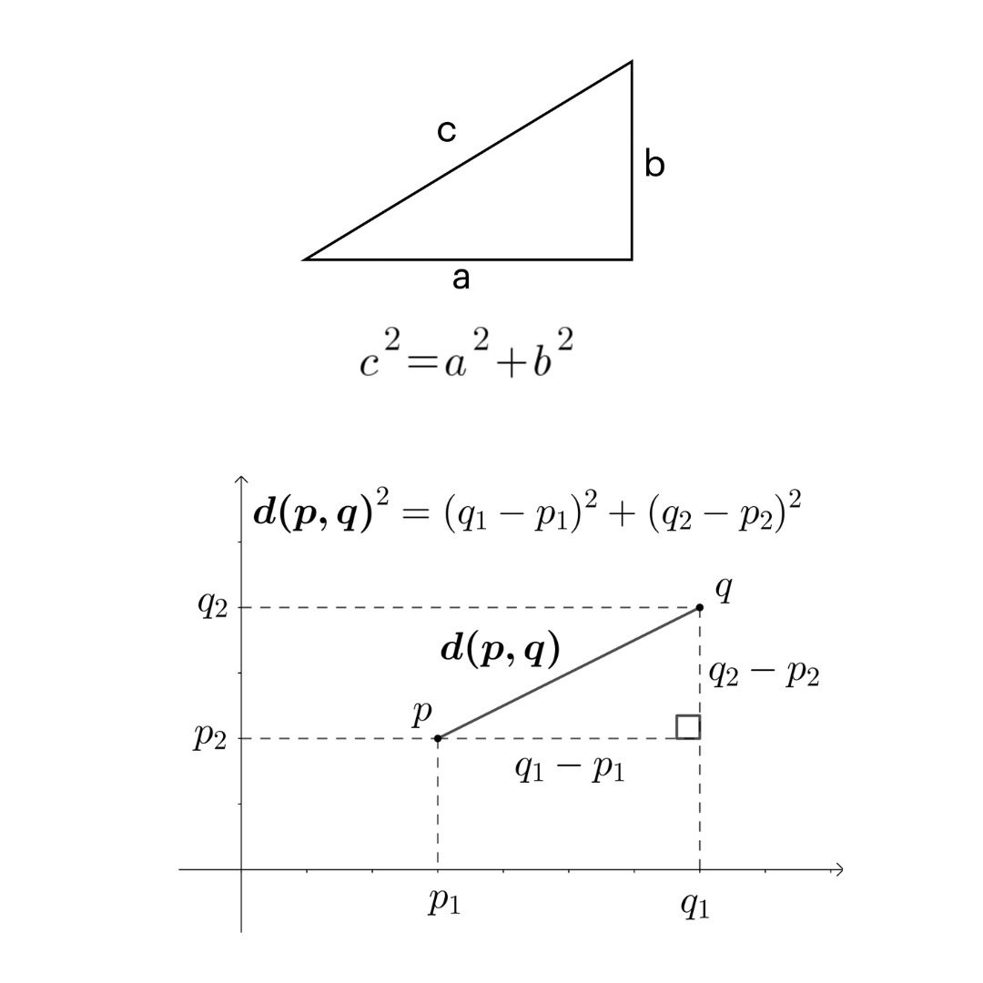
What does the Pythagorean Theorem have to do with machine learning? The Pythagorean Theorem is a formula to measure the hypotenuse of a triangle, which also allows us to calculate the distance between the origin and another point on a coordinate plane.
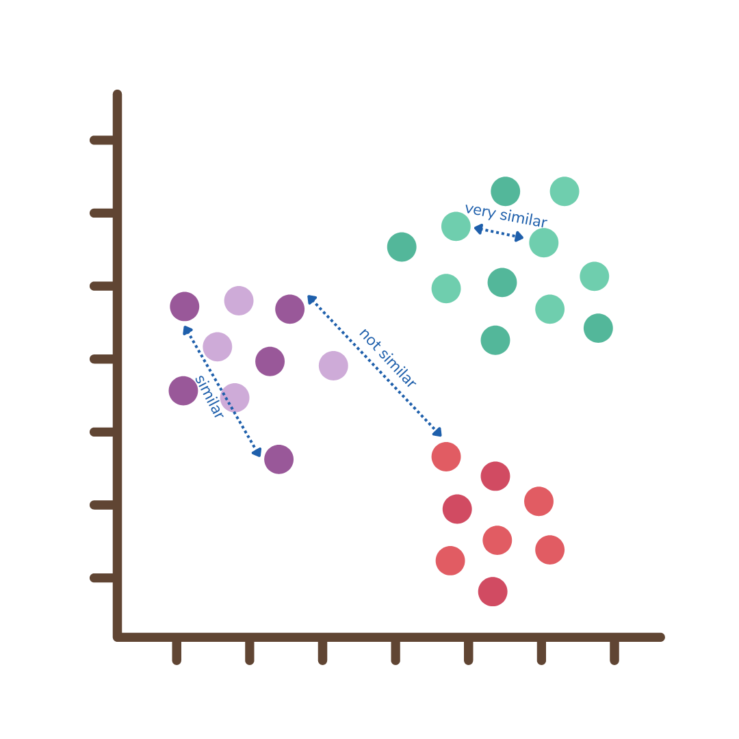
The Pythagorean Theorem can be rearranged to result in the Euclidean distance formula, to calculate the straight-line distance between any two points. The Euclidean distance metric is one of several distance metrics used in machine learning. One type of machine learning is clustering, where objects related to each other are grouped together. We can model how related objects are to each other by essentially assigning them to coordinates and calculating the distance between them; the further apart they are, the less related they are to each other.
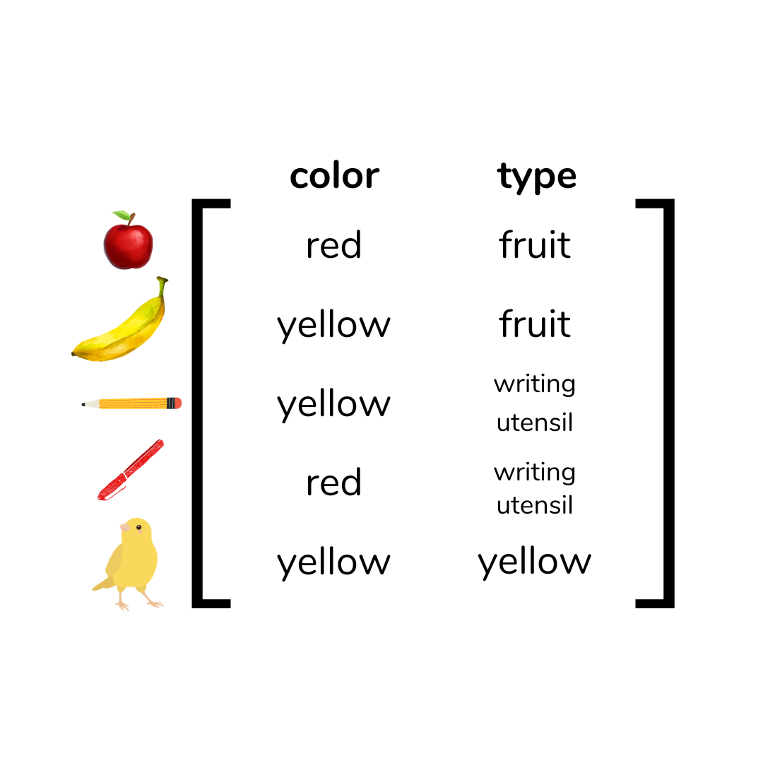
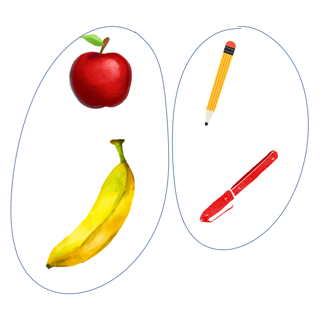
Objects can be related to each other in many different aspects. For example, say you have a red apple, a banana, a red pen, and a Number 2 pencil. How would you group these objects into two groups? You could say the apple and banana go together because they are both fruits, and the pen and pencil go together because they are both writing instruments. But you could also say that the apple and pen should go together because they are both red, and the banana and the pencil should go together because they are both yellow. In this case, you could group by type of object or by color. Grouping by type of object might make more sense in this example.
But what if we add in a canary to the things to be grouped? We want to make as many of the objects fit in the groups as possible, so the addition of a canary, which is yellow, would cause the grouping by color to make more sense.
In clustering, each of these objects would be a data point, and each aspect, such as type, color, size, and texture, would be a dimension of these objects. We call these different aspects features of the data. We can store this data in a matrix so that a computer can read and process the data.
It might seem that if we add more features to the data, we would be able to group the objects better. Intuitively, we think we have more choices of what to group by. However, as we add more and more features, the majority of features would be irrelevant and actually make it more difficult to group. This is called noise in our model. For example, one feature of the data set we had earlier could be “does it have a beak?” But since the canary is the only object that has a beak, that doesn’t help us cluster the objects together. When considering the distance between data points, adding features adds a dimension to our model, which increases the distance between points. Also, adding “does it have a beak?” as a feature would actually just increase the amount of data we have to store, making our algorithms run slower.
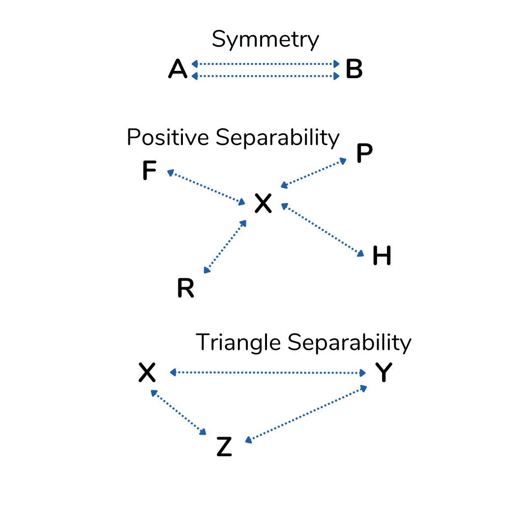
When a computer clusters data points, points within the same cluster are similar and points in different clusters are not as similar. We quantify similarity using distance metrics. There are some properties of similarity that have to hold true for clustering to make sense:
Symmetry: The distance from A to B is equal to the distance from B to A. This makes sense because if A is similar to B, B must be similar to A. Similarity goes both ways.
Positive Separability: The distance from X to X is equal to 0, and the distance from X to any other point does not equal 0. This rule is needed because a data point cannot be different from itself, and if data points are different, they have to have a distance between them representing that difference.
Triangle Separability: The distance from X to Y is less than or equal to the sum of the distance from X to Z and Y to Z. This makes sense because if Y is similar to Z, and X is similar to Z, then X must be similar to Y.
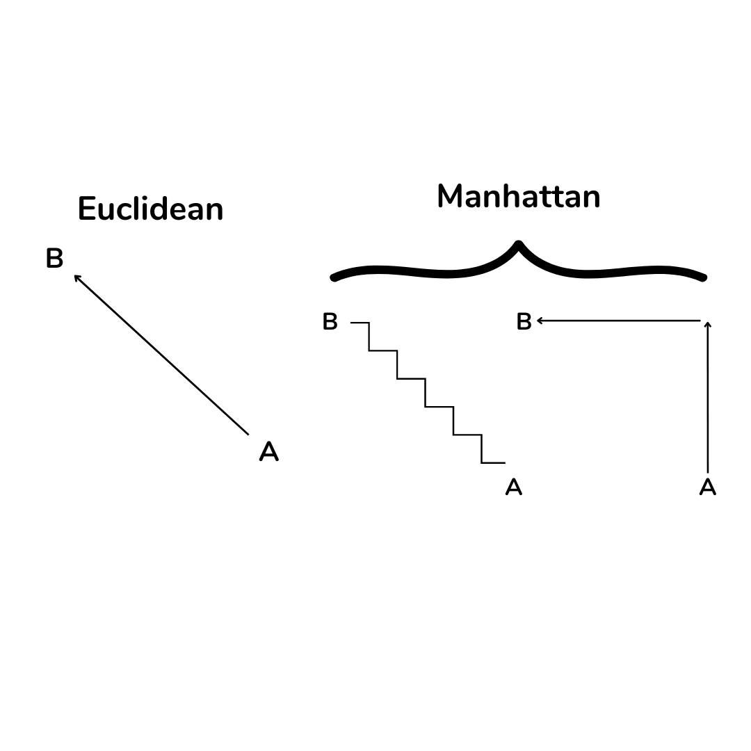
Euclidean distance is the straight-line distance from point A to point B, but here’s an example of another distance metric. Manhattan distance measures around blocks, resembling the route a car in a city would take around ceilings.
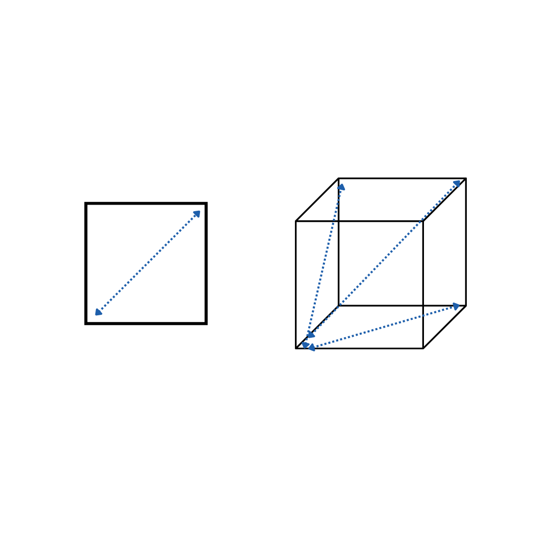
An interesting phenomenon related to distance metrics is how they lose their meaning in higher dimensions. When we add features to our dataset and increase the number of dimensions, the average distance between points increases. Think about how in one dimension when we are looking at one feature, point A and B would be on a straight line, x units apart. But in two dimensions when we added another feature, if the second feature is just as far apart as the first for points A and B respectively, A and B would be sqrt(2)*x units apart. The same pattern continues when we add more and more dimensions.
As we increase dimensions and distance between points increases, the points also migrate towards the edges of the space. This is because the ratio of the limits of the space to the core of the space increases as the number of dimensions increases. Think about how a square with sides of length x has a perimeter of 4x and an area of x^2. A cube, on the other hand, with sides of length x has a surface area of 6x^2 and a volume of x^3. Let’s substitute 1 as x to compare these values.
Square perimeter = 4x = 4
Square area = x^2 = 1
Perimeter to area ratio = 4/1 = 4
Cube surface area = 6x^2 = 6
Cube volume = x^3 = 1
Surface area to volume area = 6/1 = 6
When the number of dimensions increased from 2 to 3, the ratio increased from 4 to 6. Once again, this pattern continues in higher dimensions.
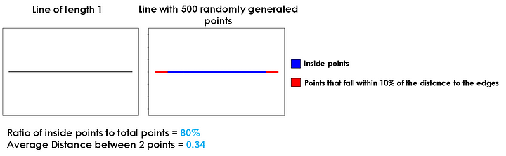
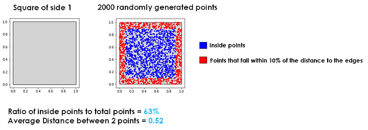
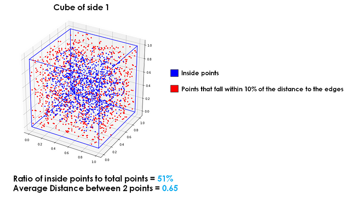
Let’s visualize a model with points randomly distributed around the model space.
In one dimension, approximately 20% of points will be within the outer 10% of the space. In two dimensions, approximately 37% of points will be within the outer 10% of the space. In three dimensions, approximately 49% of points will be within the outer 10% of the space.
Continuing on to dimensions of degrees that are essentially impossible for us to visualize, approximately 60% of points in four dimensions, 68% in five dimensions, 74% in six dimensions, and 80% in seven dimensions will be within the outer 10% of the space.
This concept brings us to the titular “infinitely-dimensional orange” concept; if we had an orange with infinity dimensions and points randomly distributed across the space, all the points would be on the peel of the orange, with no points spread around in the interior.
Using more features allows each data point to become more different from each other, which makes them more sparsely distributed. This makes it harder to cluster the points accurately! In machine learning models, we address this issue using feature selection and dimensionality reduction techniques to find the most relevant features and reduce the number of dimensions we utilize to cluster data points. Not only does this reduce the processing power a computer would need to run the algorithm, but accuracy in clustering generally also increases by preventing the “infinitely-dimensional orange” phenomenon.